Forward and Reverse KL Divergence

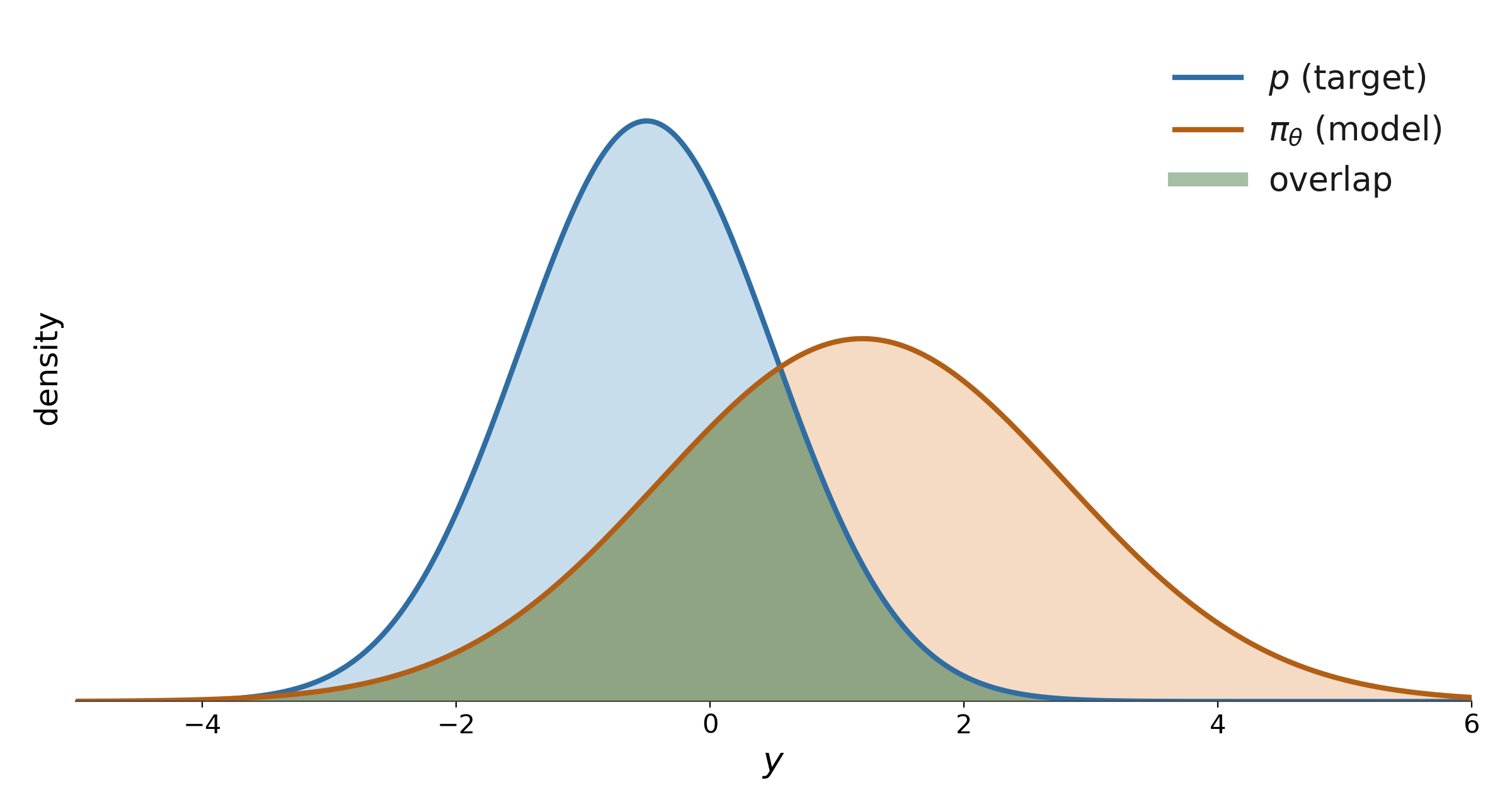
In Entropy, Prefix Codes, and KL Divergence, $D_{KL}(p|q)$ is the expected excess cost of coding a $p$ sequence with a $q$ code. It is asymmetric, and the asymmetry is the subject here. Let $p$ be a target distribution over responses $y$ and $\pi_\theta$ a model. The first argument of $D_{KL}$ is the distribution the expectation is taken over, so swapping the arguments changes what $\pi_\theta$ is forced to do. Written as expectations:

\[D_{KL}(p\|\pi_\theta) = \mathbb{E}_{y \sim p}\left[\log \frac{p(y)}{\pi_\theta(y)}\right]\] \[D_{KL}(\pi_\theta\|p) = \mathbb{E}_{y \sim \pi_\theta}\left[\log \frac{\pi_\theta(y)}{p(y)}\right]\]

This post is based on Jon Vet’s Forward and Reverse KL Divergence, following Hao (2026).¹

Forward KL

With $p$ as the first argument, the KL divergence is:

\[D_{KL}(p\|\pi_\theta) = \sum_y p(y) \log \frac{p(y)}{\pi_\theta(y)}\]

Expanding gives the cross-entropy decomposition from the earlier post:

\[\boxed{D_{KL}(p\|\pi_\theta) = -H(p) - \sum_y p(y) \log \pi_\theta(y)}\]

Proof

$$ \begin{aligned} D_{KL}(p\|\pi_\theta) &= \sum_y p(y) \log \frac{p(y)}{\pi_\theta(y)} \\ &= \sum_y p(y) \log p(y) - \sum_y p(y) \log \pi_\theta(y) \\ &= -H(p) - \sum_y p(y) \log \pi_\theta(y) \end{aligned} $$ The first sum is the negative entropy.

The expectation is over $p$, each $y$ is weighted by how often the target produces it. Fix $y$ with $p(y) > 0$ and let $\pi_\theta(y) \to 0$. The term $p(y) \log \frac{p(y)}{\pi_\theta(y)} \to \infty$. A model that gives no probability to something the target produces is penalized without bound, so $\pi_\theta$ must put mass everywhere $p$ does. This is mode-covering.

Reverse KL

Swap the arguments:

\[\boxed{D_{KL}(\pi_\theta\|p) = -H(\pi_\theta) - \sum_y \pi_\theta(y) \log p(y)}\]

Proof

$$ \begin{aligned} D_{KL}(\pi_\theta\|p) &= \sum_y \pi_\theta(y) \log \frac{\pi_\theta(y)}{p(y)} \\ &= \sum_y \pi_\theta(y) \log \pi_\theta(y) - \sum_y \pi_\theta(y) \log p(y) \\ &= -H(\pi_\theta) - \sum_y \pi_\theta(y) \log p(y) \end{aligned} $$ The first sum is the negative entropy of the model.

Both terms now depend on $\theta$. The expectation is over $\pi_\theta$ itself. If $\pi_\theta(y) \approx 0$, the term for $y$ is $\approx 0$ regardless of $p(y)$. Dropping a mode of $p$ costs nothing. If $\pi_\theta(y) > 0$ where $p(y) = 0$, the term is infinite. The support constraint is exactly reversed:

\[\boxed{D_{KL}(p\|\pi_\theta) < \infty \implies \mathrm{supp}\, p \subseteq \mathrm{supp}\, \pi_\theta}\] \[\boxed{D_{KL}(\pi_\theta\|p) < \infty \implies \mathrm{supp}\, \pi_\theta \subseteq \mathrm{supp}\, p}\]

Within the support of $p$, the average is weighted by what $\pi_\theta$ generates, so an imperfect $\pi_\theta$ does best by concentrating on the largest modes of $p$ and ignoring the rest. This is mode-seeking.

Token Precision and Recall

Forward and reverse KL can also be seen as a recall and precision tradeoff. Take $p$ as a teacher and $\pi_\theta$ as a student, both generating tokens. Run an experiment, the teacher generates a set of tokens $A$ and the student generates a set of tokens $B$. Precision and recall are the usual set quantities:

\[\mathrm{Precision} = \frac{|A \cap B|}{|B|}\] \[\mathrm{Recall} = \frac{|A \cap B|}{|A|}\]

Let’s assume we are using nucleus sampling with high temperature and top-p and tokens are sampled from the raw probability distributions.

Take the information retrieval task of picking key entities from a chunk of text. Our goal is to modify the student to maximize the average overlap over many such generations. If we optimized for forward KL, we’d find that student generations broadly cover teacher generations (recall). Student generations would generate fewer false negatives but with more false positives. If we instead optimized for reverse KL, the student would become more careful, only generating tokens it’s confident the teacher also generates (precision). We’d see fewer false positives, but more false negatives.

Maxima are achieved at the same two inclusions from when KL divergence is finite:

\[\boxed{\mathrm{Recall} = 1 \iff A \subseteq B}\] \[\boxed{\mathrm{Precision} = 1 \iff B \subseteq A}\]

Proof

Recall is $|A \cap B| / |A|$, which equals $1$ exactly when $A \cap B = A$, i.e. when $A \subseteq B$. Precision is $|A \cap B| / |B|$, which equals $1$ exactly when $A \cap B = B$, i.e. when $B \subseteq A$.

When optimized, forward KL achieves recall and reverse KL achieves precision.

Post-Training Methods

The two directions are, up to constants, the losses of the standard post-training methods. Methods differ in which divergence is optimized, and in who supplies the samples it is averaged over.

SFT

The data is a fixed set of tokens drawn from $p$, and the loss is their negative log likelihood under the model:

\[\mathcal{L}_{SFT} = -\sum_y p(y) \log \pi_\theta(y)\]

By the Forward KL expansion:

\[\boxed{\mathcal{L}_{SFT} = H(p) + D_{KL}(p\|\pi_\theta)}\]

$H(p)$ does not depend on $\theta$, so SFT is forward KL minimization. The pull is toward $p$ regardless of where the model starts, the recall direction, covering the target at the cost of the model’s prior modes. This is one of the explanations of catastrophic forgetting in LLM post-training.

KL-Regularized RL

The objective maximizes expected reward subject to staying near a frozen reference policy $\pi_{ref}$:

\[J(\theta) = \sum_y \pi_\theta(y)\, r(y) - \beta D_{KL}(\pi_\theta\|\pi_{ref})\]

Define the reward-tilted distribution:

\[p^*(y) = \frac{\pi_{ref}(y) \exp(r(y)/\beta)}{Z}\] \[Z = \sum_{y'} \pi_{ref}(y') \exp(r(y')/\beta)\]

$\pi_{ref}$ is not itself the target; together with $r$ it defines the tilted target. Then:

\[\boxed{J(\theta) = -\beta D_{KL}(\pi_\theta\|p^*) + \beta \log Z}\]

Proof

$$ \begin{aligned} D_{KL}(\pi_\theta\|p^*) &= \sum_y \pi_\theta(y) \log \frac{\pi_\theta(y)}{p^*(y)} \\ &= \sum_y \pi_\theta(y) \left[ \log \frac{\pi_\theta(y)}{\pi_{ref}(y)} - \frac{r(y)}{\beta} + \log Z \right] \\ &= D_{KL}(\pi_\theta\|\pi_{ref}) - \frac{1}{\beta} \sum_y \pi_\theta(y)\, r(y) + \log Z \end{aligned} $$ Multiplying by $-\beta$ and adding $\beta \log Z$ gives $J(\theta)$.

$\beta \log Z$ does not depend on $\theta$, so maximizing reward with a KL penalty is minimizing the reverse KL to that tilted target. The model is graded only on responses it generates.

On-Policy Distillation

On-policy distillation keeps the teacher of SFT but the sampling of RL. Responses are drawn from the student $\pi_\theta$ and scored by a teacher $\pi_T$. Its reverse KL loss, at sequence level:

\[\mathcal{L}_{OPD} = \sum_y \pi_\theta(y) \left[ \log \pi_\theta(y) - \log \pi_T(y) \right] = D_{KL}(\pi_\theta\|\pi_T)\]

The loss is reverse KL by definition. The difference from RL is the signal; a teacher log probability per generated token, instead of a scalar reward and a reference policy.

Off Policy

The data is drawn from another distribution $\mu$ (a teacher’s samples, an older checkpoint, a fixed dataset). Matching $\pi_\theta$ to it by likelihood gives:

\[\mathcal{L}_{OFF} = -\sum_y \mu(y) \log \pi_\theta(y) = H(\mu) + D_{KL}(\mu\|\pi_\theta)\]

So off-policy training is a forward KL problem toward whoever generated the data (expectation is over $\mu$). It is possible to recover an on-policy expectation from off-policy training with the importance ratio:

\[\mathbb{E}_{y \sim \pi_\theta}[f(y)] = \mathbb{E}_{y \sim \mu}\left[ \frac{\pi_\theta(y)}{\mu(y)} f(y) \right]\]

The weights grow as the model drifts away from $\mu$, which is why practical methods clip them, or refresh the data and stay near on-policy.

Summary

The direction of a KL divergence is a statement about who supplies the average. Forward KL averages over the target, so the model must become the target everywhere the target has mass. Reverse KL averages over the model, so the model must only be target-like where it already goes. That gives covering versus seeking, and is one proposed mechanism for SFT forgetting more than RL. It is not the whole story, the experiments discussed by Vet and Hao find that on-policy data itself reduces forgetting even when the KL penalty is weakened or its direction changed. The sampling distribution is a separate mechanism from the direction of the divergence.

References

• W. Hao. SFT, RL, and On-Policy Distillation Through a Distributional Lens, 2026.
• R. Agarwal et al. On-Policy Distillation of Language Models: Learning from Self-Generated Mistakes, 2024.
• H. Chen et al. Retaining by Doing: The Role of On-Policy Data in Mitigating Forgetting, 2026.

1. Logs are natural in the post-training literature. Nothing below depends on the base. ↩︎