Link Budget

Link Budget

The link budget in its most general form is,

\[P_{RX} (\text{dBm}) = P_{TX} (\text{dBm}) + G (\text{dB}) - L (\text{dB})\]

Where $P_{(\cdot)}$ is power expressed in decibels-milliwatt, $G_{(\cdot)}$ is gain expressed in decibels, $TX$ is transmitter, and $RX$ is receiver. Dimensionally, this equation balances since dBm and dB are both dimensionless units. But more specifically, they represent different ratios:

\[10\log_{10}{\frac{\text{P mW}}{\text{1 mW}}} = 10\log_{10}{\frac{\text{P mW}}{\text{1 mW}}} + 10\log_{10}{\frac{P}{P_0}} -10\log_{10}{\frac{P}{P_0}}\]

The link budget is a theoretical tool that allows you to compute how much power is “left over” from a transmission to be decoded by the receiver. Typically we have a pre-specified link margin that acts as a buffer between the received power strength and the lowest usable power. For example, if you were shopping for a radio transmitter (watts provided by manufacturer) and antenna with a specified gain (dB provided by manufacturer) over a set distance (calculated with the free space path loss equation: $L_{FS} (dB) = 20\log_{10}{4 \pi \frac{\text{distance}}{\text{wavelength}}}$) with known obstructions (dB using a list of reference values), you could calculate the anticipated power at the receiver. If the anticipated power is under the threshold for it to be usable (aka smaller than the link margin), you can adjust the physical setup (i.e. add transmission power or move the antenna) until you have enough reception to complete the communication.

Power (Decibels-Milliwatt)

dBm is power relative to 1 milliwatt in a circuit. There are other variants such as dBW (watts) and dBV (volts) but dBm is commonly used for radio systems. For a lot of household applications, this value is negative. WiFi receivers for example can receive up to -10 dBm of transmitted power. If we wanted to work out the power for the WiFi, it would be:

\[\begin{align} \text{dBm} &= 10\log_{10}{\frac{\text{P mW}}{\text{1 mW}}} \\ 10 ^ {\text{dBm} / 10} &= {\frac{\text{P mW}}{\text{1 mW}}} \\ \text{P mW} &= \text{1 mW} \cdot 10 ^ {\text{dBm} / 10} \end{align}\]

Which works out to be $10 ^ {-1} = 0.1 \text{mW} = 100 \mu\text{W}$. LoRa receivers are anywhere between -120 dBm (f watts) to -40 dBm (nano watts) in my experience. The smallest you can go (0W) would then be $-\infty$ dBm ($10 ^ {-\infty} = 0$). dBm is used for both receiving and transmitting a signal. For example the maximal transmission power for a ham radio station is 62 dBm (or 1.588 kW). An easy way to remember this is to use dBm anytime milliwatts are an appropriate comparison (i.e. electrical circuits).

Why logarithms?

Logarithms allow us to quickly compare power values on different orders of magnitude. For example, if we wanted to compare the strongest WiFi signal against the weakest LoRa signal we’d have to calculate $100 \mu\text{W} / 1\text{fW}$ which would involve tracking a lot of zeros. Using dBm however, it simplifies:

\[\begin{align} \log{100 \mu\text{W} / 1\text{fW}} &= \log{100 \mu\text{W}} - \log{1\text{fW}} \\ &= \log{100 \mu\text{W}} - \log{1 \text{mW}} - \log{1\text{fW}} + \log{1 \text{mW}} \\ &= (\log{100 \mu\text{W}} - \log{1 \text{mW}}) - (\log{1\text{fW}} - \log{1 \text{mW}}) \\ &= \log{\frac{100\mu\text{W}}{1\text{mW}}} - \log{\frac{1\text{fW}}{1\text{mW}}} \\ &= -40\text{dBm} - -120\text{dBm} \\ &= 80\text{dBm} \end{align}\]

So a ratio of two different orders of magnitude becomes a difference of -40 and -120. To convert logarithmic units back to power ratio values we can either use a chart or remember:

• 10 dBm = 10x
• 6 dBm $\approx$ 4x
• 3 dBm $\approx$ 2x
• 1 dBm = 1.259x
• 0 dBm = 1x

Just remember it’s not a linear scale i.e. 10 dBm + 10 dBm $\neq$ 20x (20 dBm is actually a 100x increase or $10 \log_{10}{100}$).

Gain (Decibels)

dB is relative to some reference power level $P_0$. For antennas, $P_0$ is measured along a certain directionality; Isotropic, Omnidirectional, Directional, Sector. $P_0$ is always measured along the axis of maximal emission. Isotropic (denoted as dBi) is very important because it models a theoretical antenna radiating uniformly in all directions (here $P_0$ can be measured along any axis because all directions are the same). Here is a visualization of different directionalities:

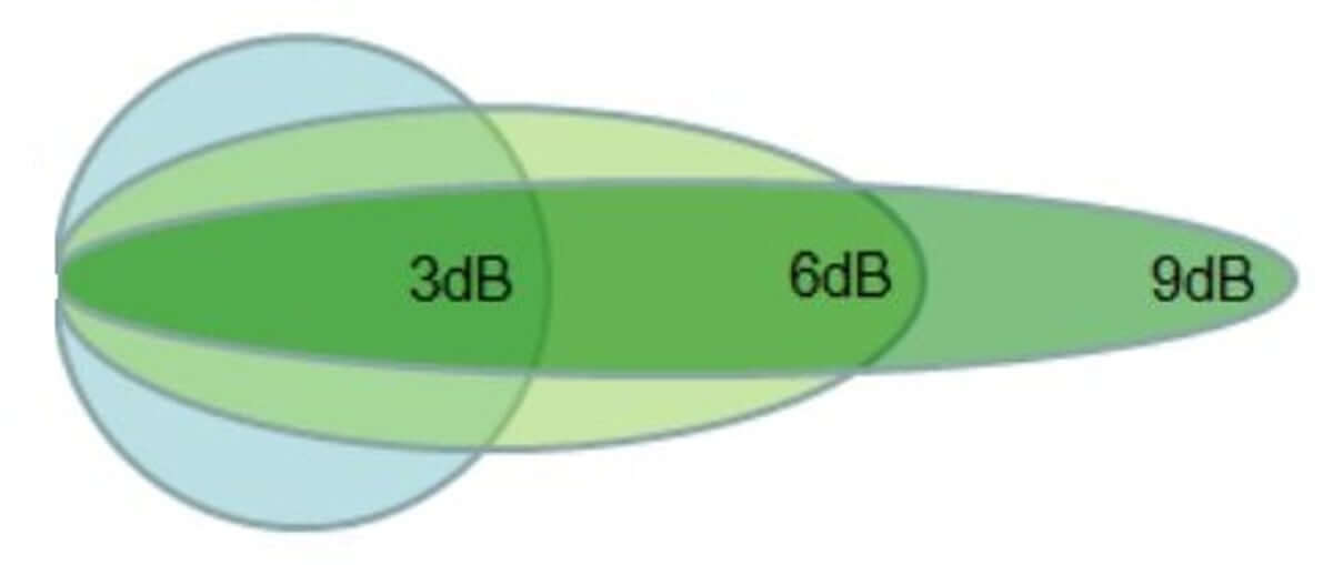
As you can see, not all antenna’s are created equal. They redistribute the existing power from the transmitter in different ways. Generally, the higher the dBi the more “focused” the radiation pattern (but lower overall coverage). The lower the dBi the lower the “focus” of the radiation pattern (but higher coverage). A 0 dBi antenna is equal to the theoretical isotropic antenna which has maximal coverage in all directions. Here are some common dBi values:

• 17cm LoRa antenna: $\approx$ 2 dBi
• Indoor WiFi antennas: 4-9 dBi
• Fiberglass omnidirectional antenna: 5.8 dBi
• Outdoor omnidirectional antennas: 6-12 dBi
• Yogi antenna: 12-18 dBi
• Point-to-point dish antenna: 18-24 dBi

Signal to Noise Ratio (SNR)

At the end of the day, the goal of any communications system is to decode a signal. In order to do that, you need to receive a signal that is louder than the prevailing background noise (I usually see a noise floor of -120 dBm for LoRa). So its sensible to calculate the power relative to this minimum threshold of being able to decode the message:

\[SNR (\text{dB}) = 10 \log_{10}{\frac{P}{P_\epsilon}}\]

Where $\epsilon$ is being used to denote noise. In this case, it is typical to see positive dB values (a negative SNR would indicate our signal is weaker than the noise!). A good SNR ratio for LoRa applications is >12 dB. To achieve this SNR value we would need to have a high received signal strength indicator (RSSI) which measures the strength of the received signal. Using our logarithm rules, we can compute it to be:

\[\text{SNR} = P (\text{dBm}) - P_\epsilon (\text{dBm}) \implies P (\text{dBm}) = 12 \text{dB} + -120 \text{dBm} = -108 \text{dBm}\]

Link Budget Example

Putting everything together, we can compute a link budget for a LoRa radio on 910.525 MHz. The maximum transmission power of a LoRa radio is 22 dBm (158mW). We can assume we have a fiberglass omnidirectional 5.8 dBi antenna using a 50ft 240 grade low-loss shielded coax cable (4 dB) for both transmitting and receiving. Assume the transmitting/receiving antennas see each other line of sight, have the same vertical polarization, and other loss sources are minimal. We will be transmitting over a distance of 5km:

\[\begin{align} L_{FS} &= 20 \log_{10}{4\pi \frac{5\text{km}}{910.525 \text{MHz}}} \\ &\approx 32.45 \text{dB} + 20 \log_{10}(910.525 \text{MHz}) + 20 \log_{10}(5 \text{km}) \\ &= 105.615 \text{dB} \end{align}\]

Now we can calculate the link budget:

\[\begin{align} P_{RX} (\text{dBm}) &= P_{TX} (\text{dBm}) + G (\text{dB}) - L (\text{dB}) \\ &= P_{TX} + G_{TX} - L_{TX} - L_{FS} + G_{RX} - L_{RX} \\ &= P_{TX} + 2 G_{TX} - 2L_{TX} - L_{FS} \\ &= 22 + 2 * 5.8 - 2 * 4 - 105.615 \\ &\approx -80 (\text{dBm}) \end{align}\]

Using a noise floor of -120 dBm, we expect to see a SNR of:

\[SNR (\text{dB}) = -80 (\text{dBm}) - -120 (\text{dBm}) = 40 (\text{dB})\]