A post about modeling tabular datasets using Undirected Graphical Models with a python package called pgmpy.
1
2
3
4
5
6
7
8
9
10
11
12
13
14
15
16
17
18
19
20
21
22
23
| import numpy as np
import pandas as pd
import plotly.graph_objects as go
import plotly.express as px
from IPython.display import display, Markdown
import itertools
from pprint import pprint
import scipy
import networkx as nx
def print_markdown(markdown: str) -> None:
display(Markdown(markdown))
def render_plotly_html(fig: go.Figure) -> None:
fig.show()
display(
Markdown(
fig.to_html(
include_plotlyjs="cdn",
)
)
)
|
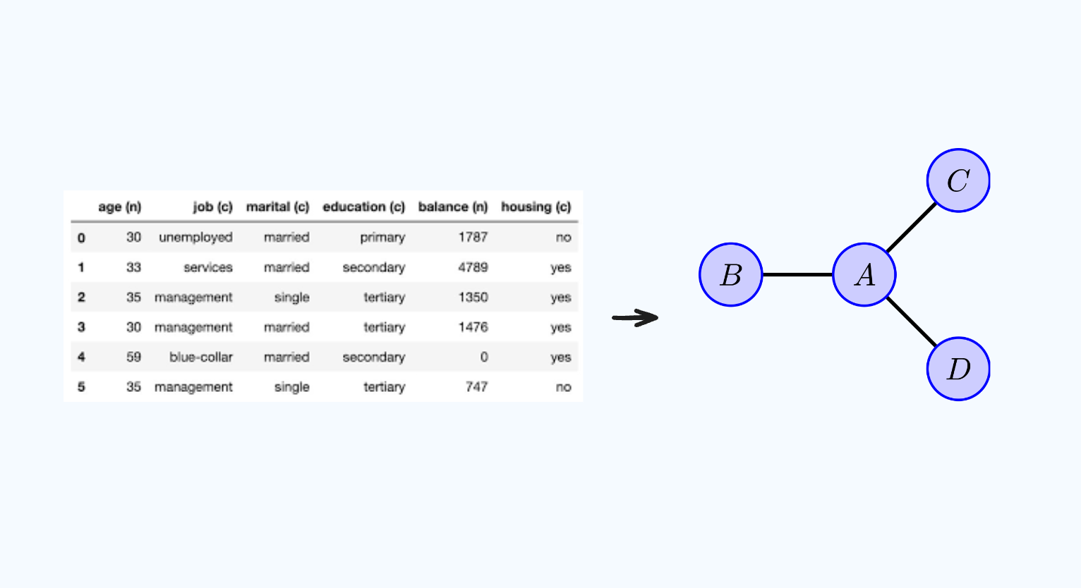
Representation
First, lets discuss tabular or relational data, that is, data that can be stored in a table. Then, I will show how we can represent this tabular dataset in an Undirected Graphical Model. I will use the adult dataset from uci repo as an example.
1
2
| X = pd.read_csv("adult.csv").fillna(value="NA")
n, p = X.shape
|
1
| print_markdown(X.head().to_markdown())
|
| | age | workclass | fnlwgt | education-num | marital-status | occupation | relationship | race | sex | capital-gain | capital-loss | hours-per-week | native-country | income>50K |
|---|
| 0 | 23 | 5 | 4 | 12 | 2 | 8 | 3 | 0 | 1 | 2 | 0 | 39 | 0 | 0 |
| 1 | 34 | 1 | 4 | 12 | 0 | 4 | 2 | 0 | 1 | 0 | 0 | 12 | 0 | 0 |
| 2 | 22 | 0 | 13 | 8 | 1 | 6 | 3 | 0 | 1 | 0 | 0 | 39 | 0 | 0 |
| 3 | 37 | 0 | 15 | 6 | 0 | 6 | 2 | 4 | 1 | 0 | 0 | 39 | 0 | 0 |
| 4 | 12 | 0 | 22 | 12 | 0 | 5 | 0 | 4 | 0 | 0 | 0 | 39 | 12 | 0 |
Histograms
One compact representation of tabular data is by a histogram. The univariate histogram is the empirical distribution of a variable:
\[\tilde P(\text{Occupation} = j) = \frac{1}{N}\sum_N I\{x_{i, \text{occupation}} = j\}\]
1
| render_plotly_html(px.histogram(X, x="occupation"))
|
Histograms can also express marginal distributions between multiple variables:
\[\tilde P(\text{Sex} = k, \text{Occupation} = j) = \frac{1}{N}\sum_N I\{x_{i, \text{sex}} = k, x_{i, \text{occupation}} = j\}\]
This will be a 2-dimensional structure, however, we can always “unroll” the counts into one long vector:
1
2
3
4
5
6
| render_plotly_html(
px.histogram(
x=X["sex"].map(str) + " / " + X["occupation"].map(str),
labels={"x": "Sex / Occupation"},
)
)
|
In this way, we can compute joint histograms of as many variables as we wish (i.e. 3, 4, …). We can also compute marginal distributions conditioned upon another variable (also known as conditional distributions):
\[\tilde P(\text{Occupation}=j \mid \text{Sex}=k)=\frac{\tilde P(\text{Occupation}=j,\text{Sex}=k))}{\tilde P(\text{Sex}=k)}\]
1
| render_plotly_html(px.histogram(X, x="occupation", facet_row="sex"))
|
Undirected Graphical Models
For discrete data like the adult dataset, histograms directly correspond to marginal distributions or marginals. The name marginal refers to the fact that these counts were often computed “in the margins” of a table. Marginal distributions are naturally modeled by Undirected Graphical Models (UGM). You can think of a UGM as a graph data structure specifically designed for storing probability distributions. UGMs factor a joint distribution into several cliques, each clique representing an unnormalized probability distribution called a factor:
\[\begin{gather*} P(x_1, ..., x_n) = \frac{1}{Z}\prod_{c \in C} \phi_c(x_c), \\ Z = \sum_{x_1, ..., x_n} \prod_{c \in C} \phi_c(x_c) \end{gather*}\]
$Z$ is a normalization constant to ensure that the joint distribution sums to 1. Internally, a factor is just a function that maps configurations of that factor’s scope to nonnegative values:
\[\begin{equation*} \phi(x_1, x_2) = \begin{cases} 10 & x_1 = x_2\\ 5 & x_1 \neq x_2\\ 1 & \text{otherwise} \end{cases} \end{equation*}\]
To model a tabular dataset with a UGM, we can add a factor for each marginal we care to measure from our dataset. For example, we might be interested in modeling the joint distribution:
\[\begin{gather*} P(\text{age}, \text{race}, \text{marital-status}, \text{education}, \text{sex}) = \frac{\phi(\text{age}, \text{race}, \text{marital-status}) \cdot \phi(\text{marital-status}, \text{education}, \text{sex})}{Z} \end{gather*}\]
We can visualize this UGM by adding a node for each clique. Edges are drawn between cliques with shared variables (i.e. marital-status) which is known as a separation set or sepset:
flowchart TD
    A(age, race, marital-status) ---|marital-status| B(marital-status, education, sex)
Factored Representations
Why is it important to factor the distribution like this? Why not just express all the variables (age, race, marital-status, education, sex), in one large clique instead of two parts:
flowchart TD
A(age, race, marital-status, education, sex)
An important consideration in modeling a tabular dataset with a UGM is the size of each clique’s state space, the space of all possible states. First, compute the # of distinct values of each column:
1
2
3
4
| # Print out the number of unique values associated with this dataset.
print_markdown(
X.nunique().rename("Unique Values").sort_values(ascending=False).to_markdown()
)
|
| | Unique Values |
|---|
| hours-per-week | 96 |
| fnlwgt | 77 |
| age | 74 |
| capital-loss | 48 |
| native-country | 42 |
| capital-gain | 23 |
| education-num | 16 |
| occupation | 15 |
| workclass | 9 |
| marital-status | 7 |
| relationship | 6 |
| race | 5 |
| sex | 2 |
| income>50K | 2 |
Taking our example from above, we would need to allocate an array of size 82,880 for $\phi(\text{age}, \text{race}, \text{marital-status}, \text{education}, \text{sex})$:
Certainly, if we tried to include every variable it becomes exponentially large:
It turns out, the way we factored the joint distribution $P(\text{age}, \text{race}, \text{marital-status}, \text{education}, \text{sex})$ into two factors (i.e. $\phi(\text{age}, \text{race}, \text{marital-status})$ and $\phi(\text{marital-status}, \text{education}, \text{sex})$) is very important for making operations on a UGM tractable.
When using UGMs to model tabular datasets it is important to limit the product of the cardinality of the individual factors. If you wish to model several columns, consider “factoring” the joint distribution into smaller factors, only including variables that are highly dependent on each other in a specific factor.
pgmpy’s FactorDict has a utility function to convert a tabular dataset into a dictionary of factors. We can use this to calculate the size of hypothetical graphical models for different factorizations. First, lets start with no factorization at all (i.e. one large clique with all the variables):
1
2
3
4
5
6
7
8
9
10
| from pgmpy.factors import FactorDict
# Model all of the variables in one large clique.
empirical_factor = FactorDict.from_dataframe(
df=X,
marginals=[
("age", "race", "marital-status", "education-num", "sex"),
],
)
pprint(empirical_factor)
|
1
| {('age', 'race', 'marital-status', 'education-num', 'sex'): <DiscreteFactor representing phi(age:74, race:5, marital-status:7, education-num:16, sex:2) at 0x16c28b9b0>}
|
1
2
3
4
5
6
| # Compute total size (measured in # of states) of the empirical marginals
np.prod(
empirical_factor[
("age", "race", "marital-status", "education-num", "sex")
].cardinality
)
|
Which matches the calculation we made above. We can also investigate a particular subset of the variables in a DiscreteFactor (through the marginalize operation). For example, if we wanted to know the empirical distribution of sex and race then:
1
2
3
4
5
6
7
8
9
10
11
| sex_race_empirical = empirical_factor[
("age", "race", "marital-status", "education-num", "sex")
].marginalize(
[
"age",
"marital-status",
"education-num",
],
inplace=False,
)
print(sex_race_empirical)
|
1
2
3
4
5
6
7
8
9
10
11
12
13
14
15
16
17
18
19
20
21
22
23
| +---------+--------+-----------------+
| race | sex | phi(race,sex) |
+=========+========+=================+
| race(0) | sex(0) | 13027.0000 |
+---------+--------+-----------------+
| race(0) | sex(1) | 28735.0000 |
+---------+--------+-----------------+
| race(1) | sex(0) | 517.0000 |
+---------+--------+-----------------+
| race(1) | sex(1) | 1002.0000 |
+---------+--------+-----------------+
| race(2) | sex(0) | 185.0000 |
+---------+--------+-----------------+
| race(2) | sex(1) | 285.0000 |
+---------+--------+-----------------+
| race(3) | sex(0) | 155.0000 |
+---------+--------+-----------------+
| race(3) | sex(1) | 251.0000 |
+---------+--------+-----------------+
| race(4) | sex(0) | 2308.0000 |
+---------+--------+-----------------+
| race(4) | sex(1) | 2377.0000 |
+---------+--------+-----------------+
|
These are “empirical marginals” in the sense that they are equal to the histogram we would have computed for $\tilde P(\text{race}, \text{sex})$. Indeed, sampling from these histograms would be the same as sampling with replacement from the original dataset which is itself equivalent with the Non-Parametric Bootstrap.
But lets assume that 82880 is too large to fit into memory on our machine. Now, lets compute a factored representation of the same variables:
1
2
3
4
5
6
7
8
| factors = FactorDict.from_dataframe(
df=X,
marginals=[
("age", "race", "marital-status"),
("marital-status", "education-num", "sex"),
],
)
pprint(factors)
|
1
2
| {('age', 'race', 'marital-status'): <DiscreteFactor representing phi(age:74, race:5, marital-status:7) at 0x311c62f60>,
('marital-status', 'education-num', 'sex'): <DiscreteFactor representing phi(marital-status:7, education-num:16, sex:2) at 0x175a3d1c0>}
|
Which models the interaction of (age, race) & (education-num, sex) through the common variable marital-status. We can compute the sum of the clique’s sizes:
1
2
| # Compute total size (measured in # of states) of the clique tree.
sum(np.prod(v.cardinality) for k, v in factors.items())
|
We can see a savings of 1 - 2814 / 82880 ~ 96% when making this conditional independence assumption!
References
Maximum Likelihood Estimates
We have talked about how to represent a probability distribution with a UGM and the tradeoffs between graph structure and memory consumption. Now, we will discuss fitting a factored UGM to a dataset and how “close” we are to the unfactored representation.
1
2
3
| from pgmpy.inference.ExactInference import BeliefPropagation
from pgmpy.estimators import MaximumLikelihoodEstimator
from pgmpy.models import JunctionTree
|
First, lets create a JunctionTree with the same nodes from our factors from before (Section 20.4 of Machine Learning - A Probabilistic Perspective). Instead of using the empirical counts as the potentials, lets compute the MLE of the factors.
1
2
3
4
5
6
7
8
9
10
| junction_tree = JunctionTree()
# Same nodes from factor.
junction_tree.add_nodes_from(factors.keys())
# Add factors, except set all the factors to the identity factor.
junction_tree.add_factors(*[i.identity_factor() for i in factors.values()])
# Add edges between the two nodes.
junction_tree.add_edge(*list(factors.keys()))
# Use `check_model` to ensure required properties of junction tree.
assert junction_tree.check_model()
print_markdown(nx.to_pandas_edgelist(junction_tree).to_markdown())
|
| | source | target | weight |
|---|
| 0 | (‘age’, ‘race’, ‘marital-status’) | (‘marital-status’, ‘education-num’, ‘sex’) | |
To fit the parameters of a JunctionTree with Maximum Likelihood, we can use an approach called Iterative Proportional Fitting. For the special case of a Junction Tree, this algorithm converges in a single iteration (Section 19.5.7 of Machine Learning - A Probabilistic Perspective).
1
2
3
| # Create estimator.
mle = MaximumLikelihoodEstimator(model=junction_tree, data=X)
mle
|
1
| <pgmpy.estimators.MLE.MaximumLikelihoodEstimator at 0x3271e1550>
|
1
2
| junction_tree.clique_beliefs = mle.get_parameters()
pprint(junction_tree.clique_beliefs)
|
1
2
| {('age', 'race', 'marital-status'): <DiscreteFactor representing phi(age:74, race:5, marital-status:7) at 0x3102e34d0>,
('marital-status', 'education-num', 'sex'): <DiscreteFactor representing phi(marital-status:7, education-num:16, sex:2) at 0x3262de8d0>}
|
With our MLE factors, we can now use the model to perform marginal inference on the sex and race variables.
1
2
3
| sex_race_query = BeliefPropagation(model=junction_tree).query(variables=["race", "sex"])
modeled_marginals = sex_race_query.values.flatten()
labels = list(str(i) for i in itertools.product(*sex_race_query.state_names.values()))
|
1
2
3
4
5
6
7
8
9
10
11
12
13
14
15
16
17
18
19
20
21
22
23
| plot_df = pd.DataFrame(
{
"Type": ["Modeled"] * len(modeled_marginals)
+ ["Observed"] * len(modeled_marginals)
+ ["Rel Diff"] * len(modeled_marginals),
"Labels": labels * 3,
"Marginals": list(modeled_marginals * n)
+ list(sex_race_empirical.values.flatten())
+ list(modeled_marginals * n / sex_race_empirical.values.flatten() - 1.0),
}
)
fig = px.bar(
plot_df,
x="Labels",
y="Marginals",
facet_row="Type",
text_auto=True,
color=np.where(plot_df["Marginals"] < 0, "red", "green"),
color_discrete_map={"red": "red", "green": "green"},
)
# fig.update_traces(marker_color=)
fig.update_yaxes(matches=None)
render_plotly_html(fig)
|
1
| 1 - np.average(np.abs(modeled_marginals * n / sex_race_empirical.values.flatten() - 1))
|
On average we “preserved” >92% of the empirical counts of the original dataset, while only using ~4% of the memory consumption. We can also compute the Jensen Shannon Divergence between the modeled & empirical counts:
1
2
3
| scipy.spatial.distance.jensenshannon(
modeled_marginals, sex_race_empirical.values.flatten() / n
)
|
Where Jensen Shannon Divergence is between 0 and 1, with 0 indicating highest similarity and 1 indicating lowest similarity.
References
Optimization
pgmpy also has a MirrorDescentEstimator that uses a proximal method and convex optimization to estimate potential values. For completeness, I include this as well even though it did not perform as well as MaximumLikelihoodEstimator.
1
| from pgmpy.estimators import MirrorDescentEstimator
|
1
2
3
4
5
6
7
8
| # Reset the same junction tree to identity factors.
junction_tree.clique_beliefs = FactorDict(
{k: v.identity_factor() for k, v in junction_tree.clique_beliefs.items()}
)
# Setup the MirrorDescentEstimator
mirror_descent = MirrorDescentEstimator(model=junction_tree, data=X)
# Estimate potential values based off the L1 distance between the modeled & empirical marginals.
junction_tree = mirror_descent.estimate(marginals=factors, metric="L1", iterations=200)
|
1
| 0%| | 0/200 [00:00<?, ?it/s]
|
1
2
3
| sex_race_query = BeliefPropagation(model=junction_tree).query(variables=["race", "sex"])
modeled_marginals = sex_race_query.values.flatten()
labels = list(str(i) for i in itertools.product(*sex_race_query.state_names.values()))
|
1
2
3
4
5
6
7
8
9
10
11
12
13
14
15
16
17
18
19
20
21
22
23
| plot_df = pd.DataFrame(
{
"Type": ["Modeled"] * len(modeled_marginals)
+ ["Observed"] * len(modeled_marginals)
+ ["Rel Diff"] * len(modeled_marginals),
"Labels": labels * 3,
"Marginals": list(modeled_marginals * n)
+ list(sex_race_empirical.values.flatten())
+ list(modeled_marginals * n / sex_race_empirical.values.flatten() - 1.0),
}
)
fig = px.bar(
plot_df,
x="Labels",
y="Marginals",
facet_row="Type",
text_auto=True,
color=np.where(plot_df["Marginals"] < 0, "red", "green"),
color_discrete_map={"red": "red", "green": "green"},
)
# fig.update_traces(marker_color=)
fig.update_yaxes(matches=None)
render_plotly_html(fig)
|
Repeat the quality metrics. It seems the MirrorDescentEstimator does not perform as well as the MaximumLikelihoodEstimator, but is still able to compress most of the statistical relationships with 4% of the parameters.
1
| 1 - np.average(np.abs(modeled_marginals * n / sex_race_empirical.values.flatten() - 1))
|
1
2
3
| scipy.spatial.distance.jensenshannon(
modeled_marginals, sex_race_empirical.values.flatten() / n
)
|
References
Summary
In this post I talked about tabular datasets and how we can model their marginals with UGMs. UGMs have the ability to factor, allowing them to express a joint distribution with less parameters. We can learn potential values for a UGM using MaximumLikelihoodEstimator and MirrorDescentEstimator, all with the pgmpy library. We saw that an estimated UGM becomes a compact representation of the table’s joint distribution.
1
2
3
4
5
6
7
8
9
10
11
12
13
| import subprocess
_ = subprocess.run(
[
"jupyter",
"nbconvert",
"--to",
"markdown",
"--output",
"~/Documents/jakee417.github.io/_includes/tabular.md",
"tabular.ipynb",
],
)
|