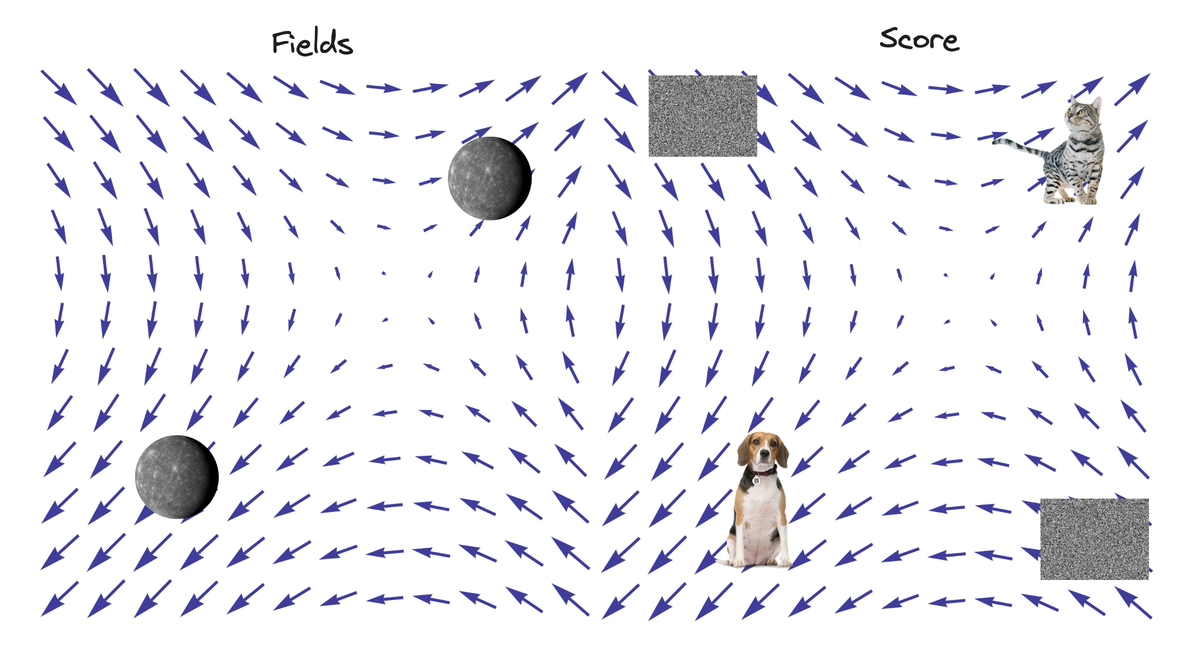
Score Functions and Field Theory

A post on the connection between the score of a likelihood function and a (scalar) field from classical field theory.

Scores and Fields

Before talking about how a field is similar to a score, I’ll first briefly review their definitions.

Fields

Scalar Field

A field is denoted with the symbol $\phi$ and is a function of a time coordinate and a collection of space coordinates,

\[\begin{equation*} \phi(t, X^i) \end{equation*}\]

Where $i$ runs from $1, 2, 3$ making the total dimensionality of the system 4-dimensional (1 time coordinate + 3 spatial coordinates).

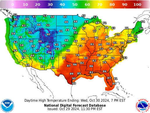
A mapping is probably the best way to describe a field. Why? Because in some cases, it is literally a map. Consider the case where $\phi$ represents the temperature along the surface of the earth at a particular point in time. We can set $t = 0$ and $X^3 = 0$ to indicate that we have frozen time at some instant of time at an elevation of zero. If we were to plot this scalar field along all $[X^1, X^2] \in \mathbb R^2$, it might look something like this:

Scalar Field $\rightarrow$ Scalar Field

Fields can also create other fields. For example, the map above is measured in degrees fahrenheit, but there is an equivalent map defined in degrees celsius:

\[\begin{equation*} \phi_{\text{Celsius}}(t, X^i) = \frac{5}{9} (\phi_{\text{Fahrenheit}}(t, X^i) - 32) \end{equation*}\]

And of course fields can be composed of more complicated functions of other fields,

\[\phi = \phi_1 * \phi_2 + \phi_3 + \phi_4^2 + \log{\phi_5}\]

Despite the added complexity, $\phi$ will still look like our simple weather map from above.

Vector Fields

So far, I have described a $\phi$ that is scalar valued:

\[\phi: (t, X^i) \rightarrow \mathbb R\]

where the output is a single number (i.e. temperature). $\phi$ can also be vector valued:

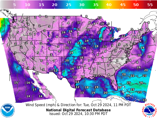
\[\phi: (t, X^i) \rightarrow \mathbb R^p\]

where the output is itself multi-dimensional. An example where $\phi$ is vector valued (keeping the weather analogy) would be a wind velocity map. For example, surface winds measured at some snapshot in time can be described by the field, $\phi: (0, X^1, X^2, 0) \rightarrow \mathbb R^2$:

Instead of each $(t, X^i)$ telling us a single quantity, each point now describes 2 numbers: wind velocity in the $X^1$ and $X^2$ directions (adding these vectors together would be the resulting arrows in the wind map above). Now $\phi$ has components itself:

\[\phi_{\text{Wind Velocity}}(t, X^i) = [\phi^{1}(t, X^i), \phi^{2}(t, X^i)]\]

Scalar Fields $\rightarrow$ Vector Fields

We can start with a scalar field and do some operation to get a vector field. For example, taking the derivatives with respect to each of the components:

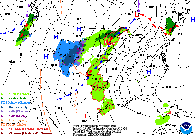
\[\frac{\partial \phi}{\partial X^\mu} = \big (\frac{\partial \phi}{\partial t}, \frac{\partial \phi}{\partial X^1}, \frac{\partial \phi}{\partial X^2}, \frac{\partial \phi}{\partial X^3} \big ) = \nabla_{X} \phi\]

This operation $\nabla_X(\cdot)$ is called the Jacobian and for a scalar valued function, results in a vector field of partial derivatives. Let’s take $\phi$ to be the temperature again, i.e. a scalar field. If we find the differences amongst its spatial coordinates $\big (\frac{\partial \phi}{\partial X^1}, \frac{\partial \phi}{\partial X^2}, \frac{\partial \phi}{\partial X^3} \big)$, we can draw surface fronts of hot air / cold air differences:

Vector Fields $\rightarrow$ Scalar Fields

Can we go the other way? We can take our velocity vector field and convert it back to a scalar field. To convert velocity into wind speed (which is the magnitude of each of the velocity vectors) we use the operation:

\[\phi_{\text{Wind Speed}}(t, X^i) = \sqrt{\phi^{1}(t, X^i)^2 + \phi^{2}(t, X^i)^2}\]

The name of this operation is the Euclidean Norm. It combines the components of a vector in a way that is invariant to translations and rotations. Another example would be the Divergence of a field which uses the Jacobian from before:

\[\text{div } \phi = \nabla \cdot \phi = \frac{\partial \phi}{\partial X^1} + \frac{\partial \phi}{\partial X^2} + \frac{\partial \phi}{\partial X^3}\]

Which describes how each point of the field’s flux acts as a source point. Using the rule for vector addition, we can see that divergence is just the composite vector resulting from the sum of the partial derivatives of the scalar field.

In summary, fields are “maps” from coordinates to either values or vectors. We can combine them to create more complicated fields and switch back and forth between scalar fields and vector fields.

A Physics Field

Now lets take an unknown field $\phi$ that is interacting with a point particle at rest. Here is the Lagrangian of this physical system:

\[\mathcal L = \frac{1}{2} \big [(\frac{\partial \phi}{\partial t})^2 - (\frac{\partial \phi}{\partial X^1})^2 - (\frac{\partial \phi}{\partial X^2})^2 - (\frac{\partial \phi}{\partial X^3})^2 \big ] - g \rho(X^i) \phi(t, X^i)\]

If the Lagrangian is new to you, check out my earlier post here. We can understand it by breaking down the components:

• $\phi(t, X^i)$ now represents an unknown scalar field. Our goal is to solve for this term and understand how it influences the point particle.
• $\frac{\partial \phi}{\partial t}$, $\frac{\partial \phi}{\partial X^1}$, $\frac{\partial \phi}{\partial X^2}$, & $\frac{\partial \phi}{\partial X^3}$ are the components of the Jacobian of $\phi$. Similar to how we computed wind speed earlier, we are now computing the difference of squares between the time and spatial components.
• Why the difference of squares in particular (i.e. Minkowski Distance)? Because it is Lorentz invariant which is important for the Lagrangian to be compatible with the theory of special relativity.
• $\rho(X^i)$ is a source function that depends only on the position of some point particle. Since $X^i$ represents the entirety of our spatial coordinates, we can “pick out” a rest point by taking $\rho(X^i) = \delta^3 (X^i)$ where $\delta^3 = \delta(X^1)\delta(X^2)\delta(X^3)$ is the three dimensional dirac function with the property:

\[\int F(x)\delta(x)dx = F(0)\]

• $g$ is a coupling constant which measures the strength of the field upon the point particle. This is simply a number that is independent of the field $\phi$ or the point particle.

We have already seen all of these operations; squaring fields, adding fields, and multiplying fields by constants. Based off the rules from above, $\mathcal L$ will still be a scalar field.

If you’d like to see a detailed derivation of $\mathcal L$ starting from the basic $L = T - V$ Lagrangian Mechanics formulation, see Chapter 5 of Special Relativity and Classical Field Theory by Leonard Susskind and Art Friedman.

Equations of Motion

$\mathcal L$ does not yet tell us how a particle would behave in the field. To find the equations of motion we have to apply the Euler Lagrange equations. Euler Lagrange finds a unique $\phi$ such that the action is stationary (i.e. minimized):

\[\begin{gather*} \text{Action} = \int \mathcal L d^4 x \\ \\ \stackrel{\text{stationary soln}}{\rightarrow} \sum_\mu \frac{\partial}{\partial X^\mu} \frac{\partial L}{\partial (\frac{\partial \phi}{\partial X^\mu})} = \frac{\partial L}{\partial \phi} \end{gather*}\]

The calculation is:

\[\begin{gather*} \frac{\partial}{\partial X^i} \frac{\partial L}{\partial (\frac{\partial \phi}{\partial X^i})} = \frac{\partial}{\partial X^i} \frac{\partial \phi}{\partial X^i} \\ = \frac{\partial^2 \phi}{\partial (X^i)^2} \end{gather*}\]

Which holds for all spatial coordinates $i$ and also $t$:

\[\frac{\partial ^2 \phi}{\partial t^2} - \frac{\partial^2 \phi}{\partial (X^1)^2} - \frac{\partial^2 \phi}{\partial (X^2)^2} - \frac{\partial^2 \phi}{\partial (X^3)^2} = \frac{\partial L}{\partial \phi}\]

And the right hand side is, $\frac{\partial L}{\partial \phi} = -g\rho(X^\mu) = -g\delta^3(X^\mu)$ which gives the equation of motion:

\[\frac{\partial ^2 \phi}{\partial t^2} - \frac{\partial^2 \phi}{\partial (X^1)^2} - \frac{\partial^2 \phi}{\partial (X^2)^2} - \frac{\partial^2 \phi}{\partial (X^3)^2} = -g\delta^3(X^\mu)\]

In our special case, remember that the particle is at rest. Therefore it is reasonable to seek a static solution and we can set $\frac{\partial ^2 \phi}{\partial t^2} = 0$:

\[\begin{gather*} \frac{\partial^2 \phi}{\partial (X^1)^2} + \frac{\partial^2 \phi}{\partial (X^2)^2} + \frac{\partial^2 \phi}{\partial (X^3)^2} = g\delta^3(X^\mu) \\ \implies \nabla^2 \phi = g\delta^3(X^\mu) \end{gather*}\]

Where $\nabla^2(\cdot)$ is called the Laplace operator and is shorthand for the sum of the second partial derivatives of the scalar field.

Physics Examples

This equation can be recognized as Poisson’s equation which describes a variety of physical systems (with coupling constant $g$ having several forms):

• Electrostatics $\nabla^2 \phi = \rho(X^\mu) / \epsilon_0$ is the electric potential with electric charge density $\rho(X^\mu)$.
• Gravitation $\nabla^2 \phi = 4\pi G \rho(X^\mu)$ is the gravitational potential with mass density $\rho(X^\mu)$.

$\nabla^2 \phi = \rho(X^\mu) / \epsilon_0$ is compatible with the Electrostatic equations using $\pmb E = -\nabla \phi$ for the electric field, $\pmb B$ for the magnetic field, and $\pmb J$ for the current field:

\[\begin{gather*} \nabla \cdot \pmb E = \frac{\rho}{\epsilon_0} \\ \nabla \cdot \pmb B = 0 \\ \nabla \times \pmb E = 0 \\ \nabla \times \pmb B = \mu_0 \pmb J \end{gather*}\]

Which is a special case of Maxwell’s equations which describe a moving electric charge:

\[\begin{gather*} \nabla \cdot \pmb E = \frac{\rho}{\epsilon_0} \\ \nabla \cdot \pmb B = 0 \\ \nabla \times \pmb E = -\frac{\partial \pmb B}{\partial t} \\ \nabla \times \pmb B = \mu_0(\pmb J + \epsilon_0 \frac{\partial \pmb E}{\partial t}) \end{gather*}\]

Going back to the general equations of motion, if we drop the requirement that $\frac{\partial ^2 \phi}{\partial t^2} = 0$, then we arrive at Diffusion Equations:

• Diffusion Equation $\frac{\partial \phi}{\partial t} - k \nabla^2 \phi = S(X^\mu)$ is the diffusion of a solute as it interacts with a source $S(X^\mu)$ and diffusion constant $k$.
• Heat Diffusion Equation $\frac{\partial T}{\partial t} - \kappa \nabla^2 T = (\rho c)^{-1}S(X^\mu)$ describes the temperature field $T(t, X^\mu)$ as it diffuses with a density $\rho$, specific heat $c$, coefficient of thermal diffusivity $\kappa = \frac{k}{\rho c}$, and source of heat $S(X^\mu)$.

The specific form of the Lagrangian, $\mathcal L$, results in a variety of physical examples.

A Statistics Field

Probability Density Function

A score is based off a probability density function involving a random vector $X^n \in \mathbb R^n$ and a vector of parameters $\theta^m \in \mathbb R^m$ which models some true, but unknown, probability density function $p_{X}$:

\[\begin{gather*} p(X^n; \theta^m) = \frac{1}{Z(\theta^m)} q(X^n; \theta^m) \in \mathbb R \\ p(X^n; \theta^m) \approx p_X \end{gather*}\]

For example, we can take $n = 2$ and $m = 2$ which would be a two dimensional continuous state space ($x \in \mathbb R^2$) and a probability density function that depends on two parameters; $\mu \in \mathbb R^2$ and $M \in \mathbb R^{2 \times 2}$. The multivariate normal distribution (MVN) is given by:

\[p(X^n; M, \mu) = \frac{1}{Z(M, \mu)} \exp{\big (-\frac{1}{2}(X^n - \mu)^T M (X^n - \mu)\big )}\]

The appropriate weather analogy in this case would be the probability of precipitation: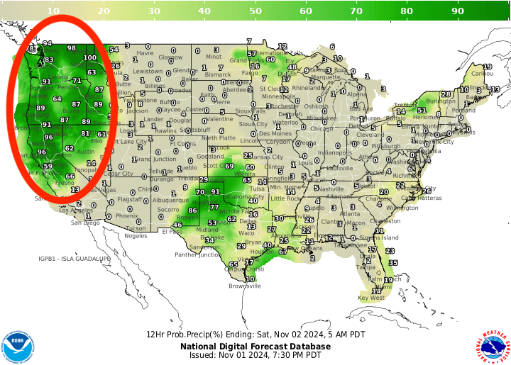

The red ellipsis (i.e. contour of a MVN) represents $p(x; M, \mu)$ and the probability of precipitation is $p_X$. In this case, $p(x; M, \mu)$ is not expressive enough to capture $p_X$ which appears to be bimodal and not elliptical.

Score Functions

In general, $Z(\theta^m)$ is intractable to compute (despite it being well known for a MVN):

\[Z(\theta^m) = \int_{X^n} q(X^n; \theta^m) dX^n\]

This is where the score function comes in:

\[\mathcal S(X^n; \theta^m) = \nabla_X \log{p(X^n; \theta^m)} \in \mathbb R^n\]

Which no longer depends on $Z(\theta^m)$:

\[\begin{gather*} \nabla_X \log{p(X^n; \theta^m)} = \nabla_X \log{ q(X^n; \theta^m)} - \nabla_X \log{Z(\theta^m)} \\ = \nabla_X \log{ q(X^n; \theta^m)} \end{gather*}\]

Some important points about $\mathcal S$ are:

• This is the Jacobian of the log probability density function with respect to the random vector $X^n$.
• The typical definition of the score function is the Jacobian with respect to the parameters $\theta^m$. Instead, we are following Hyvarinen’s paper which is with respect to the random vector $X^n$. This forms the basis of diffusion models.
• If $p(X^n; \theta^m)$ is playing the part of the scalar field from before, applying the $\log$ transforms this to a different scalar field and applying $\nabla_X$ is like converting the temperature map to the surface fronts.

Based on these observations, the score function is a vector field.

Estimating the Score Function

Similar to application of the Least Action Principle which takes a Lagrangian $\mathcal L$ and finds a unique equation of motion by finding the stationary points of the action, we need to estimate a unique score function that best describes the true score function $S_X(X^n)$.

For this, we use the score matching objective:

\[\begin{gather*} J(\theta^M) = \frac{1}{2}\int_{X^n} p_X(X^n) ||S(X^n; \theta^m) - S_X(X^n) ||^2 dX^n \\ \hat \theta^M = \arg \min_{\theta^m} J(\theta^m) \end{gather*}\]

The resemblance to the least action principle is striking. We can identify the loss function:

\[\mathcal L_{loss} = ||S(X^n; \theta^m) - S_X(X^n)||^2\]

known as Fisher Divergence playing the role of the Lagrangian from before. The Euclidean Norm operation:

\[||x||^2 = (x_1^2 + \dots + x_n^2)\]

Is very similar to the operation we used on our scalar field from the Lagrangian except before we used the Minkowski norm to be Lorentz invariant (which is not important in statistics). Following the theorems in Hyvarinen’s paper, we arrive at:

\[\begin{gather*} J(\theta^M) = \frac{1}{2}\int_{X^n} p_X(X^n) ||\mathcal S(X^n; \theta^m) - \mathcal S_X(X^n) ||^2 dX^n \\ = \int_{X^n} p_X(X^n) \sum_{i=1}^n \big [\frac{\partial}{\partial X^i} \mathcal S_i(X^n; \theta^m) + \frac{1}{2}\mathcal S_i(X^n; \theta^m)^2 \big ]dX^n + const. \\ \approx \frac{1}{T}\sum_{t=1}^T \sum_{i=1}^n \big[\frac{\partial}{\partial X^i} \mathcal S_i(X_t^n; \theta^m) + \frac{1}{2} \mathcal S_i(X_t^n; \theta^m)^2 \big] + const. \\ = \frac{1}{T} \sum_{t=1}^T \big [ \text{trace}\big(\frac{\partial}{\partial X^n}\mathcal S(X_t^n; \theta^m)\big) + \frac{1}{2}||\mathcal S(X_t^n; \theta^m)||^2 \big ] \\ = \tilde J(\theta^m) \end{gather*}\]

Where in the first step they used integration by parts to avoid the dependency on $\mathcal S_X(X^n)$ (which is unknown), the second step approximates the loss with the sample loss over a dataset of $T$ observations, and the third step expresses this in vector operations. $\tilde J$ is a consistent estimator for $J$ in that it converges in probability towards the true $\theta^m$ given infinite samples.

Score Examples

MVN Distribution

If we set $p(X^n; M, \mu)$ to a MVN:

\[p(X^n; M, \mu) = \frac{1}{Z(M, \mu)} \exp{\big (-\frac{1}{2}(X^n - \mu)^T M (X^n - \mu)\big )}\]

Then the score function is simply,

\[\mathcal S(X^n; \theta^m) = -M(X^n - \mu)\]

And the second partial is:

\[\frac{\partial}{\partial X^i} \mathcal S(X^n; \theta^m) = -m_{ii}\]

The objective function $\tilde J(M, \mu)$ becomes:

\[\tilde J(M, \mu) = \frac{1}{T} \sum_{t=1}^T \big [\sum_i -m_{ii} + \frac{1}{2}(X_t^n - \mu)^T MM (X_t^n - \mu) \big ]\]

Which is minimized (and thus the score matching estimate) if:

\[\begin{gather*} \hat \mu = \frac{1}{T}\sum_{t=1}^T X_t^n \\ \hat M = \big (\frac{1}{T}\sum_{t=1}^T (X_t^n - \mu)(X_t^n - \mu)^T \big )^{-1} \end{gather*}\]

Which matches the maximum likelihood estimate. Given a sample of data, we can estimate $\hat \mu$ and $\hat M$ and form:

\[\hat {\mathcal S}(X^n; \hat \theta^m) = -\hat M(X^n - \hat \mu)\]

Which can generate new samples using Langevin Dynamics MCMC:

\[\tilde X_t^n = \tilde X_{t-1}^n + \frac{\epsilon}{2} \hat {\mathcal S}(\tilde X_{t-1}^n; \hat \theta^m) + \sqrt{\epsilon} Z_t^n\]

For demonstration purposes, we can set $\hat \mu = [0, 0]$ and

\[\hat M^{-1} = \begin{bmatrix} 1 & 0.5 \\ 0.5 & 1 \\ \end{bmatrix}\]

And visualize the pdf, score function, and sampling process:

This is not really necessary for generating samples from a MVN, but is required for generating natural images. More complicated applications will require estimating the score function with a large neural network i.e. $s_{\theta^m}(X^n)$.

Conclusion

In physics and statistics we can:

• Define a scalar field
• Compute gradients of scalar field
• Define a function of the scalar field and it’s gradients
• Find stationary points of the function

	Fields	Score
Scalar Field	$\phi$	$p(X^n; \theta^m)$
Gradients of Scalar Field	$\frac{\partial \phi}{\partial X^\mu}$	$\mathcal S(X^n; \theta^m)$
Scalar Field & Gradients Function	Lagrangian $\mathcal L$	Loss function $J(\theta^m)$
Find Stationary Points	$\nabla^2\phi = g\delta^3(X^\mu)$	$\hat \theta^M = \arg \min_{\theta^m}J(\theta^m)$

Following this procedure yields results in both fields and it is interesting to compare and contrast how they are used.