Model Uncertainty For Linear Regression

What is model uncertainty?

Although linear regression isn’t always used to simulate data, it gives a good theoretical starting point to build intuition of why model uncertainty matters at all. We observe ($y$) depending on some covariates ($X$) and we want to “generate” synthetic $y$ values ($y_0$) at new covariate values ($x_0$). Under this setting, we can analytically compare the variation in $y_0$ compared to the variation of $y$.

\[\begin{gather} y = X\beta + \epsilon \\ \epsilon \sim \mathcal N(0, \sigma^2) \\ y|X \sim \mathcal N(X\beta,\sigma^2) \end{gather}\]

In this case, $\sigma^2$ is known as data (aleatoric) uncertainty. It is irreducible in the sense that regardless of how many observations of $X$ we have, we always have at least $\sigma^2$ noise in an estimate of $y$. To generate new data from $y$, we need to estimate $\beta$. For this we can use the least squares estimate:

\[\begin{gather} \hat \beta =(X^TX)^{-1}X^Ty \end{gather}\]

But since $\hat \beta$ is a function of $y$, $\hat \beta$ is also random and has its own sampling distribution. We refer to this sampling distribution as model (epistemic) uncertainty and is given by,

\[\begin{gather} \hat \beta | X \sim \mathcal N(\beta, (X^T X)^{-1} \sigma^2) \end{gather}\]

For illustrative purposes, consider when

\[X = \vec 1\]

i.e. when $X$ is a single intercept term. In this case,

\[\mathbb V[\hat \beta | X]= \mathbb V[\bar y | X ] = \frac{\sigma^2}{n}\]

Predictive Distribution

Using the sampling distribution of $\hat \beta$, we can reason about the predictive distribution of $y_0$ at a test point $x_0$:

\[\begin{gather} y_0 = x_0^T \hat \beta + \epsilon \\ y_0 | X, x_0 \sim \mathcal N(x_0^T \beta, c \cdot \mathbb V[y | X]) \\ c = (x_0^T(X^T X)^{-1}x_0 + 1) \end{gather}\]

Thus, $y_0$ involves both the data uncertainty of $y$ and $c = (x_0^T(X^T X)^{-1}x_0 + 1)$ which is related to the model uncertainty of estimating $\beta$. Putting this another way (and assuming $X^T X$ is invertible),

\[\begin{flalign} \frac{\mathbb V[y_0 | x] - \mathbb V[y|x]}{\mathbb V[y | X]} &= \frac{c\mathbb V[y | X] - \mathbb V[y | X]}{\mathbb V[y | X]} \\ &= c - 1 \\ &= x_0^T(X^T X)^{-1}x_0 \geq 0 \end{flalign}\]

Which means that the relative difference between the predictive and the aleatoric uncertainty will always be positive and depends on $X$ and $x_0$’s locations. For a more detailed discussion, see Linear Models with R, Section 3.5.

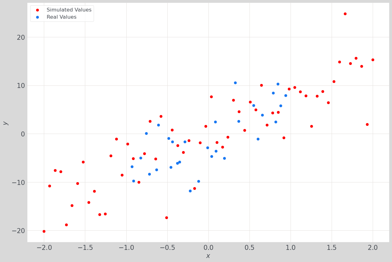
Below, we visualize real ($y$) vs. simulated data ($y_0$) for a toy dataset.

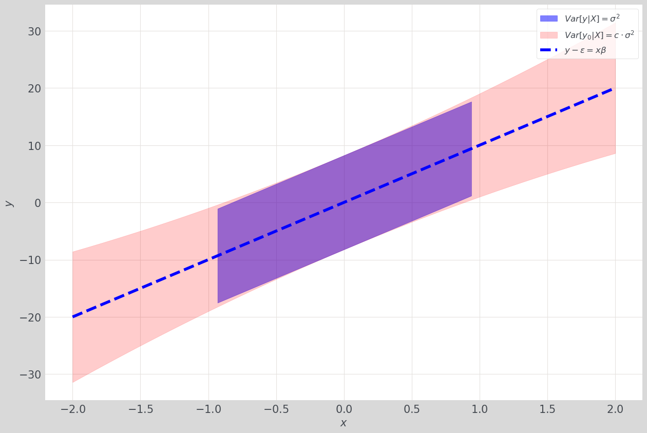
Now, we compare

\[\mathbb V[y | X] \text{ and } \mathbb V[y_0 | X]\]

pointwise around:

\[y - \epsilon = X\beta\]

Appendix

Linear model in $y$

\[\begin{gather*} y = X\beta + \epsilon \\ \epsilon \sim N(0,\sigma^2) \end{gather*}\] \[\begin{gather*} \mathbb E[y|X] = \mathbb E[X\beta + \epsilon | X] = X\beta \\ \mathbb V[y|X] = \mathbb V[\beta X + \epsilon | X] = \sigma^2 \end{gather*}\] \[\therefore y | X \sim \mathcal N(X\beta, \sigma^2)\]

Sampling distribution of $\hat \beta$

\[\hat \beta = (X^T X) X^T y\] \[\begin{flalign*} \mathbb E[\hat \beta | X] &= \mathbb E[(X^T X)^{-1} X^T y | X] \\ &= (X^T X)^{-1} X^T \mathbb E[y|X] \\ &= (X^T X)^{-1} X^T X \beta \\ & = \beta \end{flalign*}\] \[\begin{flalign*} \mathbb V[\hat \beta | X] &= \mathbb V[(X^T X)^{-1} X^T y | X] \\ &= (X^T X)^{-1} X^T \mathbb V[y | X] X(X^T X)^{-1} \\ &= \sigma^2 (X^T X)^{-1} X^T X (X^T X)^{-1} \\ &= \sigma^2(X^TX)^{-1} \end{flalign*}\] \[\therefore \hat \beta | X \sim N(\beta,(X^T X)^{-1} \sigma^2)\]

Predictive distribution of $y_0$

\[y_0 = x_0^T \hat \beta + \epsilon\] \[\begin{gather*} \mathbb E[y_0 | X, x_0] = \mathbb E[x_0^T \hat \beta + \epsilon| X, x_0] = x_0^T \beta \end{gather*}\] \[\begin{flalign*} \mathbb V[y_0 | X, x_0] &= \mathbb V[x_0^T \hat \beta + \epsilon | X, x_0] \\ &= x_0^T (X^T X)^{-1} x_0 \sigma^2 + \sigma^2 \\ &= (x_0^T (X^T X)^{-1} x_0 + 1)\sigma^2 \\ &= (x_0^T (X^T X)^{-1} x_0 + 1) \mathbb V[y|X] \\ &= c \cdot \mathbb V[y|X] \end{flalign*}\] \[\therefore y_0 | X, x_0 \sim \mathcal N(x_0^T \beta, c \cdot \mathbb V[y|X])\]

This is different from the idea of just “plugging-in” $\hat \beta$ to the equation $y_0 = x_0^T \hat \beta + \epsilon$ to draw simulated values and treating the random quantity $\hat \beta$ as fixed. This would yield,

\[y_0| \hat \beta, X \sim \mathcal N(x_0^T \beta,\mathbb V[y | X])\]

And would exclude the model’s uncertainty of the parameter $\beta$. For more details see Probabilistic Machine Learning, Section 11.7.4.