Least Action vs. Least Squares
In this post I want to describe two methods that both use the word “Least” to describe them. Both of these concepts are foundational in their respective field (physics and statistics), and I find it interesting to compare/contrast their formulation.
Path Minimization
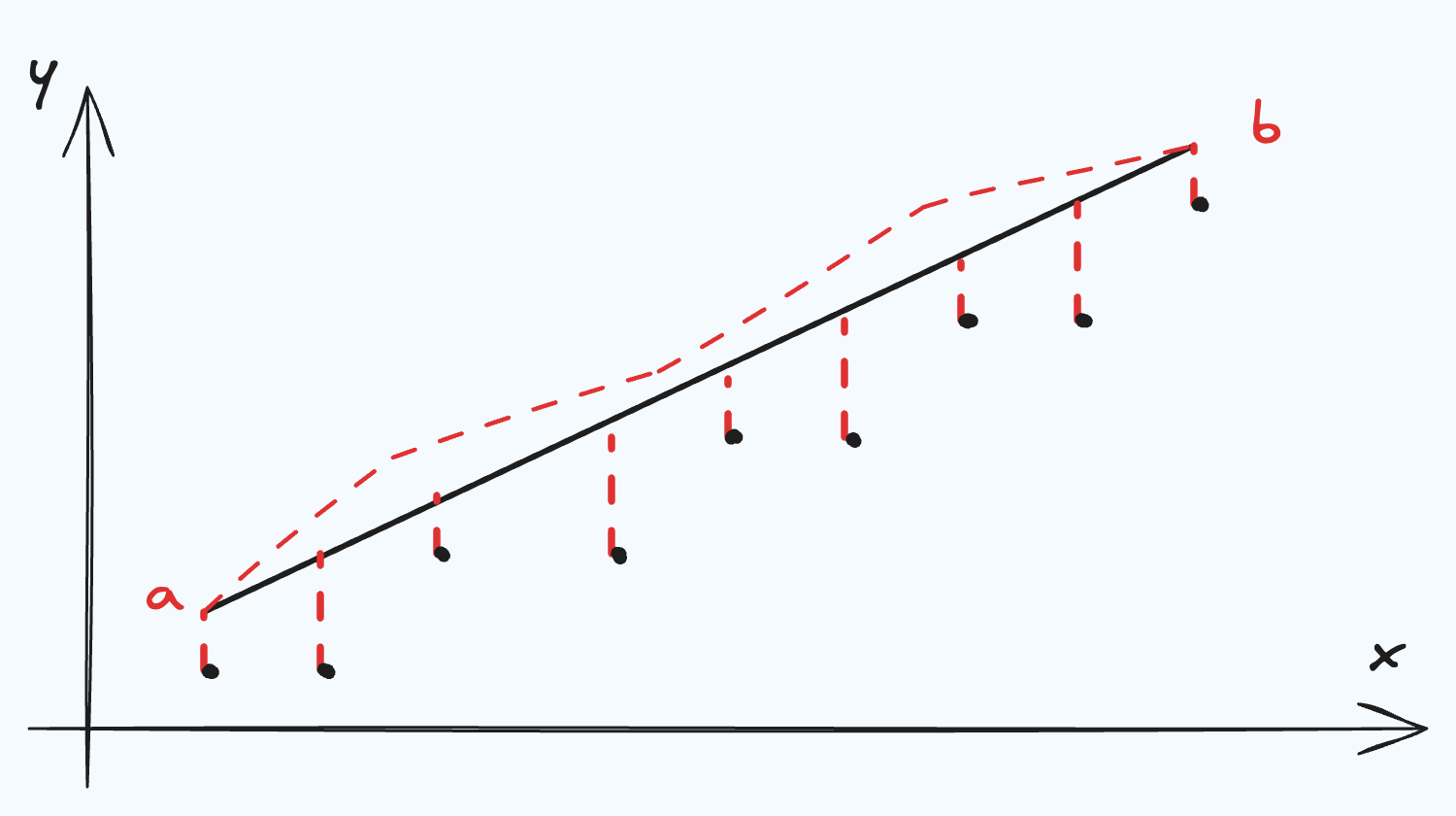
 We start with a path. A path consists of $(x, y(x))$ points in space. When we vary $x + \delta x$, we can move to the corresponding $y$ coordinate along the step defined by $y’(x) = \frac{dy}{dx}$. We can encode this entire relation inside a functional:
Which has a path integral (the “length” of the path from points $a$ to $b$) of:
\[\begin{equation*} I[y] = \int_a^b F(y(x), y'(x), x)dx \end{equation*}\]Now, if we wanted to say, minimize this path, we can consider an alternative path starting and ending at the same points ($x=a$ and $x=b$) but “perturbed” by some small amount, $\epsilon$:
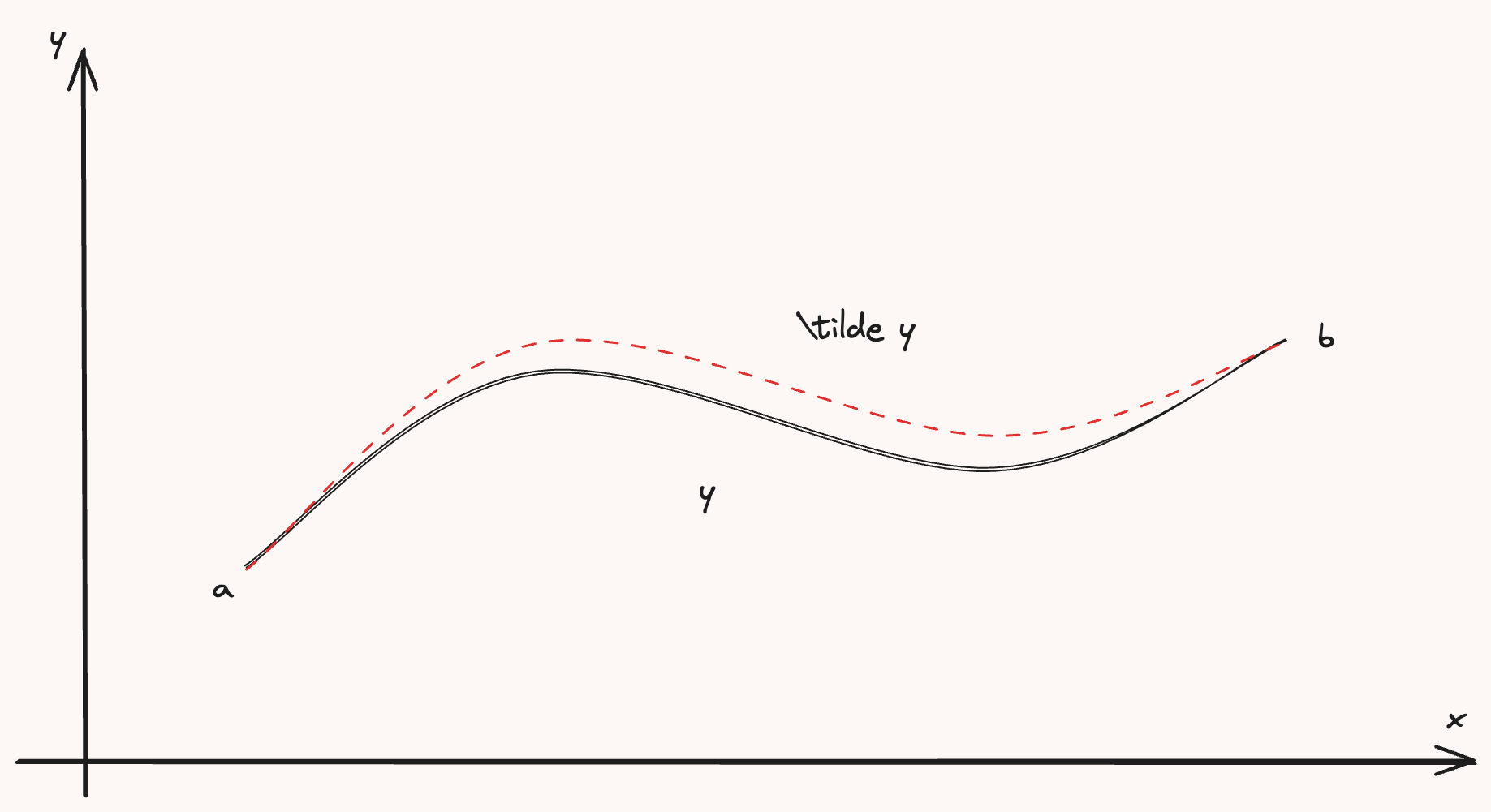
\[\tilde y(x) = y(x) + \epsilon \eta(x), \eta(a) = \eta(b) = 0\]Where $\tilde y(x)$ only differs from $y(x)$ on the interior of $[a, b]$. $\tilde y(x)$ also has a path length,
\[\begin{equation*} I[\tilde y] = \int_a^b F(\tilde y(x), \tilde y'(x), x)dx \end{equation*}\]Since $y$ and $\tilde y$ were arbitrary functions, we know that for any $\epsilon > 0$, $I[\tilde y(x)] > I[y(x)]$ because $\epsilon$ is making $\tilde y(x) > y(x)$. So to “find” the smallest version of $I[y]$, we can tighten the $\epsilon$ bound around it by minimizing:
\[\begin{gather*} \frac{dI[\tilde y]}{d\epsilon}\bigg |_{\epsilon=0} = 0 \\ \implies \int_a^b \frac{d}{d\epsilon}F(\tilde y(x), \tilde y'(x), x)\bigg |_{\epsilon=0} dx = 0 \end{gather*}\]Lets take a pause and review before the algebra. We have already defined $y(x)$ and its path from $a$ to $b$ as $I[y]$. From whichever $y(x)$ we start with, we can always find a larger version $\tilde y(x)$ which has a nonnegative component $\epsilon \eta(x)$. We are now minimizing $I[\tilde y]$ as a bound on $I[y]$, which has the affect of searching, over a space of functions, for the smallest path. Okay, onto the algebra…
First,
$\int_a^b \frac{d}{d\epsilon}F(\tilde y(x), \tilde y'(x), x)\bigg |_{\epsilon=0} dx = 0 \implies \int_a^b (\frac{\partial F}{\partial \tilde y}\eta + \frac{\partial F}{\partial \tilde y'}\eta')\bigg |_{\epsilon=0} dx = 0$
$$ \begin{flalign*} \frac{dF}{d\epsilon} &= \frac{\partial F}{\partial \tilde y} \frac{\partial \tilde y}{\partial \epsilon} + \frac{\partial F}{\partial \tilde y'} \frac{\partial\tilde y'}{\partial \epsilon} \\ &= \frac{\partial F}{\partial \tilde y} \eta + \frac{\partial F}{\partial \tilde y'} \eta' \end{flalign*} $$then,
$\int_a^b (\frac{\partial F}{\partial \tilde y}\eta + \frac{\partial F}{\partial \tilde y'}\eta')\bigg |_{\epsilon=0} dx = 0 \implies \int_a^b (\frac{\partial F}{\partial \tilde y} - \frac{\partial}{\partial x} \frac{\partial F}{\partial \tilde y'})\bigg |_{\epsilon=0} \eta dx = 0$
Use a substitution for the second term, $\frac{\partial F}{\partial \tilde y'}\eta'$ $$ \begin{flalign*} \int_a^b \frac{\partial F}{\partial \tilde y'}\eta'dx = \frac{\partial F}{\partial \tilde y}\eta \bigg |_a^b - \int_a^b \frac{\partial}{\partial x}\frac{\partial F}{\partial \tilde y'}\eta dx \end{flalign*} $$ And recognize that $\frac{\partial F}{\partial \tilde y}\eta \bigg |_a^b$ is 0 by construction ($\eta(a) = \eta(b) = 0$)And finally we are left with,
\[\begin{equation*} \frac{dI[\tilde y]}{d\epsilon} = \int_a^b (\frac{\partial F}{\partial \tilde y} - \frac{\partial}{\partial x} \frac{\partial F}{\partial \tilde y'})\bigg |_{\epsilon=0} \eta dx = 0 \end{equation*}\]which goes to zero for any functional $F$ at $\epsilon = 0$ provided that,
\[\begin{equation*} \frac{\partial F}{\partial y} - \frac{\partial}{\partial x} \frac{\partial F}{\partial y'} = 0 \end{equation*}\]By the fundamental lemma of calculus of variations. This last expression is known as the Euler Lagrange equation. By design, when following the trajectory of this second-order differential equation, you also minimize a trajectory along a path.
Least Action
Turning Path Minimization into the Least Action Principle is straightforward at this point. Replace $x \rightarrow t$, $y \rightarrow q$ and $y’ \rightarrow \dot q$:
\[\begin{equation*} A[q] = \int_{t_1}^{t_2} L(q(t), \dot q(t), t) dt \end{equation*}\]$q$ is known as a generalized coordinate representing for example cartesian or polar coordinates and $\dot q(t)$ is short-hand for the time derivative of q with respect to t, $\frac{dq}{dt}$. Here is the really cool part, when we specify $L$, we can then apply the Euler Lagrange equation to automatically find the Least Action path. The most famous example is if we let $L$ be the difference between the kinetic and potential energy and $q$ be cartesian coordinates, $L = \frac{1}{2}m \dot q^2 - V(q)$:
\[\begin{flalign*} \frac{\partial L}{\partial q} - \frac{\partial}{\partial t}\frac{\partial L}{\partial \dot q} &= 0 \\ \frac{\partial L}{\partial q} &= \frac{\partial}{\partial t}\frac{\partial L}{\partial \dot q} \\ -\frac{\partial V}{\partial q} &= \frac{\partial}{\partial t} m\dot q \\ F &= m \ddot q \end{flalign*}\]So if we use $L = T - V$, and pass that through Euler Lagrange Equations, we recover Newton’s Second Law. Equivalently, Newton’s Second Law is the exact trajectory that minimizes the action over the functional $L = T - V$.
Here is another example, but this time taking $q$ to be polar coordinates:
\[\begin{equation*} L = \frac{1}{2}m(\dot \rho^2 + \rho^2\dot\phi^2) - V(\rho) \end{equation*}\]Which yields the equation (in the $\phi$ axis):
\[\begin{equation*} \frac{\partial}{\partial t}\frac{\partial L}{\partial \dot \phi} = m\rho^2\dot\phi = 0 \end{equation*}\]Another property of the Lagrangian is that $\frac{\partial L}{\partial \dot q}$ is always the conjugate momentum, which I understand to mean a generalized form of Newton’s $p = mv$. So, $\frac{\partial L}{\partial \dot \phi}$ is equal to the (conjugate) momentum in the $\phi$ direction, $p_\phi$, implying that angular momentum is conserved with respect to time. You can see both of these examples here along with more exotic examples here.
Here is the takeaway, these physical systems only differ in the form of $L$. Once we can express the system in terms of $L$, Least Action & Euler Lagrange are a common framework to determine the equations of motions, conserved quantities, and conjugate momentum.
KL Divergence Minimization
 Now, lets switch tracks. Instead of a path between two points, lets abstract the discussion to two probability distributions. Our goal is now to find the smallest distance between two probability distributions. Instead of taking a path integral like before, we will use tools from Information Theory to define a notion of “distance”:
- Entropy - best possible long term average bits per message (optimal) that can be achieved under a symbol distribution $P(X)$ by using an encoding scheme (possibly unknown) specifically designed for $P(X)$.
I was always a little confused by this quantity until I worked out a simple example by hand. Consider the distribution:
\[P(X = x_1) = P(X = x_2) = ... = P(X = x_n) = \frac{1}{n}\]Then the entropy is (using base-$n$ for illustration):
\[\mathbb E_{x \sim P}[-\log P(x)] = n * \frac{1}{n} * -(\log_n(\frac{1}{n})) = -(-1) = 1\]So the entropy roughly measures the (weighted) average of the probability’s negative exponent. This is maximized (most random) when the negative exponent is spread uniformly across the domain. To keep comparisons fair however, we don’t change the base of the $\log$ and fix this to $e$ corresponding to the unit of measure called nats.
- Cross Entropy - long term average bits per message (suboptimal) that results under a symbol distribution $P(X)$, by reusing an encoding scheme (possibly unknown) designed to be optimal for a scenario with symbol distribution $Q(X)$.
- KL Divergence - penalty we pay, as measured in average number of bits, for using the optimal scheme for $Q(X)$, under the scenario where symbols are actually distributed as $P(X)$.
So, it seems KL divergence is a good candidate to use a notion of “distance” between two distributions (where “distance” is nominal only, since KL divergence does not satisfy the triangle inequality).
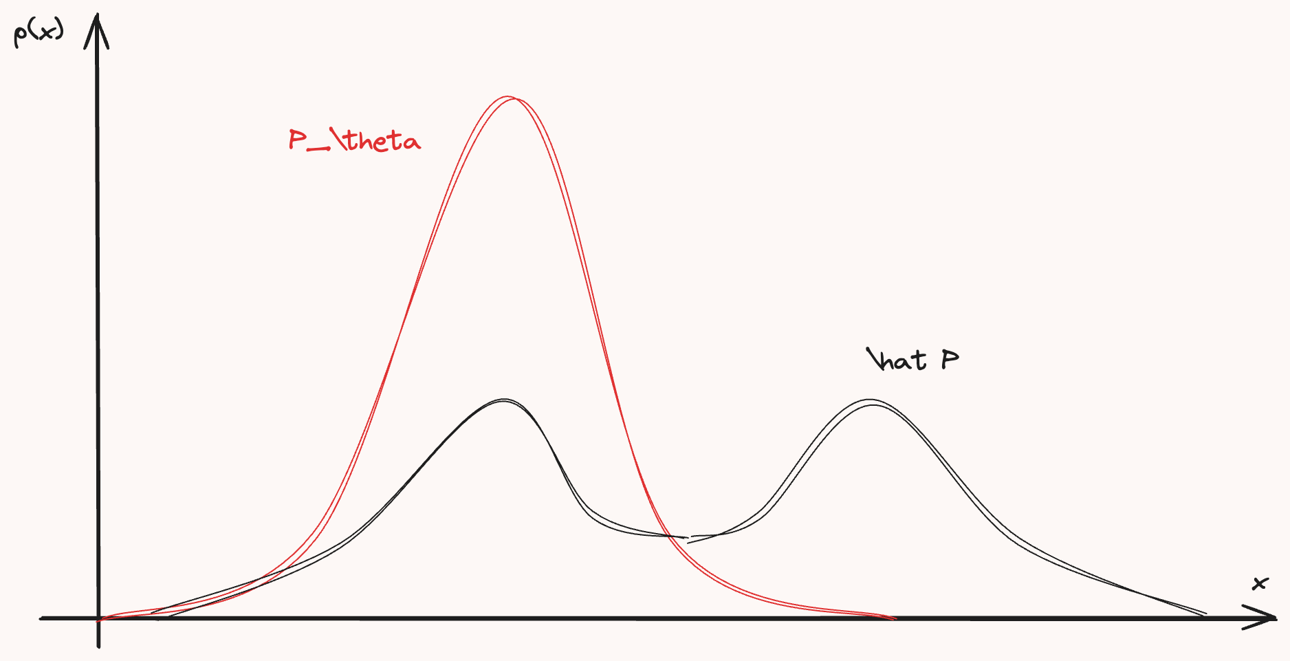
I remember from CS229 PS3, there was a problem asking us to prove that minimizing the KL Divergence between a parameterized distribution \(P_\theta\) (i.e. Normal, Bernoulli, Binomial etc.) and the empirical distribution of the population \(\hat P\), this is equivalent with maximizing likelihood estimate for \(\theta\). We are looking for single expression that, when satisfied, is equivalent with minimizing the KL divergence between two distributions:
CS 229 Problem Set 3 2.C
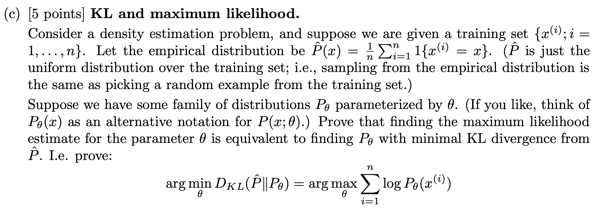
First, lets define the empirical distribution:
\[\hat P(x) = \frac{1}{n} \sum_{i=1}^n \mathbb I\{x^{(i)} = x\}\]To show the equivalence, we work from the definition of KL divergence towards something that maximizes the log-likelihood:
\[\begin{flalign*} \arg \min_\theta D_{KL}(\hat P || P_{\theta}) &= \arg \min_\theta \sum_{x \in \mathcal X} \hat P(x)\log{\hat P(x)} - \sum_{x \in \mathcal X} \hat P(x)\log{P(x)}\\ &= \arg \max_\theta \sum_{x \in \mathcal X} \hat P(x)\log{P(x)}\\ &= \arg \max_\theta \sum_{x \in \mathcal X} \frac{1}{n} \sum_{i=1}^n \mathbb I\{x^{(i)} = x\}\log{P(x)} \\ &= \arg \max_\theta \frac{1}{n} \sum_{i=1}^n \sum_{x \in \mathcal X} \mathbb I\{x^{(i)} = x\}\log{P(x)} \end{flalign*}\]The key here is that the inner sum is only nonzero for the unique value \(x \in \mathcal X\) such that \(x = x^{(i)}\). Hence,
\[= \arg \max_\theta \frac{1}{n} \sum_{i=1}^n\log{P(x^{(i)})}\]Which is the Maximum Likelihood Estimate. Similar to the Euler Lagrange Equation above, when we are able to satisfy this equation, we also minimize the KL divergence between two distributions at the same time.
Least Squares
Similar to when we replaced the lagrangian $L$ with a specific expression for Cartesian Coordinates, we now replace $P(x^{(i)})$ with a specific probability distribution. In the next two examples, consider a paired dataset, $\big (x^{(i)}, y^{(i)} \big)_{i=1}^n$. First, we hypothesize the following statistical model:
\[\begin{equation*} y^{(i)} \sim Normal(x^{(i)}\theta, \sigma^2) \end{equation*}\]Plugging this into our Maximum Likelihood Estimate equation from above:
\[\begin{flalign*} \arg \max_\theta \frac{1}{n} \sum_{i=1}^n\log{P(x^{(i)})} &= \arg \max_\theta \frac{1}{n} \sum_{i=1}^n\log{\mathcal N(y^{(i)}; x^{(i)}\theta, \sigma^2)} \\ &= \arg \max_\theta \frac{1}{n} \sum_{i=1}^n \log{\frac{1}{\sigma \sqrt{2\pi}}\exp{-\frac{1}{2}\big (\frac{y^{(i)} -x^{(i)}\theta}{\sigma} \big) ^2}} \\ &= \arg \max_\theta \frac{1}{n} \sum_{i=1}^n c - \frac{1}{2}\big (\frac{y^{(i)} -x^{(i)}\theta}{\sigma} \big) ^2 \\ &= \arg \min_\theta \frac{1}{n} \sum_{i=1}^n \big (y^{(i)} -x^{(i)}\theta\big)^2 \end{flalign*}\]Which is the Least Squares objective! Minimizing this further for $\theta$ gives the famous estimate:
\[\begin{align*} \frac{d}{d\theta} \frac{1}{n} \sum_{i=1}^n \big (y^{(i)} -x^{(i)}\theta\big)^2 &= 0 \\ \frac{1}{n} \sum_{i=1}^n -2x^{(i)} \big (y^{(i)} -x^{(i)}\theta\big) &=0 \\ \sum_{i=1}^n -x^{(i)}y^{(i)} + \sum_{i=1}^n x^{(i)}x^{(i)}\theta &= 0 \\ \implies \hat \theta = \frac {\sum_{i=1}^nx^{(i)}y^{(i)}}{\sum_{i=1}^nx^{(i)}x^{(i)}} \end{align*}\]And of course, the power of this generality is that we can swap out $P(x^{(i)})$ and quickly derive new estimators. Consider another statistical model:
\[\begin{equation*} y^{(i)} \sim Laplace(x^{(i)}\theta, b) \end{equation*}\]And taking the same steps as before:
\[\begin{flalign*} \arg \max_\theta \frac{1}{n} \sum_{i=1}^n\log{P(x^{(i)})} &= \arg \max_\theta \frac{1}{n} \sum_{i=1}^n\log{\mathcal L(y^{(i)}; x^{(i)}\theta, b)} \\ &= \arg \max_\theta \frac{1}{n} \sum_{i=1}^n \log{\frac{1}{b}\exp{-\frac{1}{2}\big |\frac{y^{(i)} -x^{(i)}\theta}{b} \big |}} \\ &= \arg \max_\theta \frac{1}{n} \sum_{i=1}^n c - \frac{1}{2}\big |\frac{y^{(i)} -x^{(i)}\theta}{b} \big | \\ &= \arg \min_\theta \frac{1}{n} \sum_{i=1}^n \big |y^{(i)} -x^{(i)}\theta\big | \end{flalign*}\]Which is the Least Absolute Deviations estimator after solving the minimization problem with a linear program.
Once again, these two estimators only differed in the probability distribution used inside the statistical model. Once we define $P(x^{(i)})$, finding the Maximum Likelihood Estimate automatically finds the “closest” distribution to the sample’s empirical distribution judged by the KL Divergence.
Lagrangians and Loss Functions
I think the comparison between Least Action and Least Squares makes the most sense in terms of hierarchy. For example, take your favorite OOP programming language and try to express each of the different concepts as classes. In pseudocode, this would look something like:
1
2
3
4
5
6
7
8
9
10
11
12
13
14
class LeastAction:
    def f(y, y_prime, x, V): ...

    def conjugate_momentum(): ...

    def conserved_quantities(): ...

class CartesianCoordinates(LeastAction):
    def f(y, y_prime, x, V):
        return (1 / 2) * m * y_prime ** 2 - V(y)

class PolarCoordinates(LeastAction):
    def f(y, y_prime, x, V):
        return (1 / 2) * m * (y_prime[0] ** 2 + y[0] ** 2 * y[1] ** 2) - V([y[0]])
And similarly for the Least Squares:
1
2
3
4
5
6
7
8
9
10
11
12
class MaximumLikelihood:
    def loss(y, y_hat): ...

    def estimate_parameters(): ...

class LeastSquares(MaximumLikelihood):
    def loss(y, y_hat):
        return sum((y - y_hat) ** 2)

class LeastAbsoluteDeviation(MaximumLikelihood):
    def loss(y, y_hat):
        return sum(abs(y - y_hat))
Once you work out the subclass’s implementation, you can rely on the parent class as a framework to do generic calculations.