Marginal Learning in Discrete Markov Networks

A x-post from my contribution to pgmpy, a library for probabilistic graphical models in python. You can find the original tutorial here, MirrorDescentEstimator here and MaximumLikelihoodEstimator here.

Marginal Learning in Discrete Markov Networks

In this notebook, we show an example for learning the parameters (potentials) of a Factor Graph or Markov Network given the data and its corresponding marginals.

In the examples, we will generate some data from given models and perform out of clique inference for certain queries.

Modeling who wins a Football game

Model who wins a football game just based off who won each game of the season.

from pgmpy.models import FactorGraph, JunctionTree
from pgmpy.factors.discrete import DiscreteFactor
import numpy as np
import networkx as nx
import pandas as pd
import itertools
from pgmpy.estimators.MLE import MaximumLikelihoodEstimator
from pgmpy.estimators import MirrorDescentEstimator
from pgmpy.inference.ExactInference import BeliefPropagation
from pgmpy.factors import FactorDict
from matplotlib import pyplot as plt

Step 1: Load the games data and form a FactorGraph

games has the results of the 2023-2024 NFL season including the playoffs, but excluding the Super Bowl.

games = pd.read_csv("examples/data/games.csv")
# Define a "win" to include ties for the home team.
games["homeWin"] = (games.homeFinalScore >= games.visitorFinalScore).map(
    lambda x: "win" if x else "loss"
)
TEAMS = sorted(set(games.homeTeamAbbr).union(set(games.visitorTeamAbbr)))
COLUMNS = ["homeTeamAbbr", "visitorTeamAbbr", "homeWin"]
df = games[COLUMNS]
df.head()

	homeTeamAbbr	visitorTeamAbbr	homeWin
0	NYG	DAL	loss
1	NYJ	BUF	win
2	NE	PHI	loss
3	BAL	HOU	win
4	MIN	TB	loss

G = FactorGraph()
nodes = COLUMNS
# Map of variables to all possible states.
state_names = {
    "homeTeamAbbr": TEAMS,
    "visitorTeamAbbr": TEAMS,
    "homeWin": ["loss", "win"],
}
cardinalities = {"homeTeamAbbr": 32, "visitorTeamAbbr": 32, "homeWin": 2}
# Form factors with all possible combinations of columns. Initialize each
# factor with zeros.
factors = [
    DiscreteFactor(
        variables=i,
        cardinality=[cardinalities[j] for j in i],
        values=np.zeros(tuple(cardinalities[j] for j in i)),
        state_names=state_names,
    )
    # Model one-way, two-way, & three-way marginals.
    for i in list(
        itertools.chain.from_iterable(
            [list(itertools.combinations(COLUMNS, i)) for i in range(1, 4)]
        )
    )
]
G.add_nodes_from(nodes=nodes)
G.add_factors(*factors)
G.add_edges_from(
    [(node, factor) for node in nodes for factor in factors if node in factor.scope()]
)
G.check_model()

True

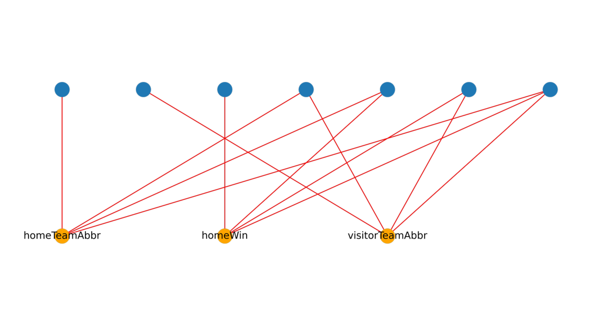
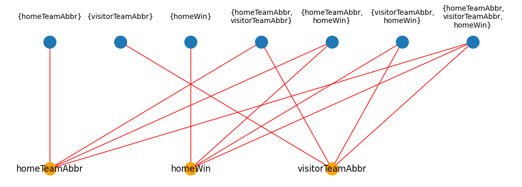
# Print the structure of the Graph to verify its correctness.
plt.figure(figsize=(10, 3))
top = {team: (i * 2, 0) for i, team in enumerate(sorted(nodes))}
bottom = {factor: (i, 1) for i, factor in enumerate(factors)}
# Draw all the variables & factors with their edges.
nx.draw(
    G,
    pos={**top, **bottom},
    edge_color="red",
)
# Draw text labels for the factors above their nodes in the graph.
label_dict = {factor: "{" + ",\n".join(factor.scope()) + "}" for factor in G.factors}
for node, (x, y) in bottom.items():
    plt.text(x, y * 1.2, label_dict[node], fontsize=10, ha="center", va="center")
# Re-draw the variables but with labels this time and colored orange.
nx.draw(
    G.subgraph(nodes),
    node_color="orange",
    pos={**top},
    with_labels=True,
)
plt.show()

Step 2: Define a model using MaximumLikelihoodEstimator

# Initialize model
estimator = MaximumLikelihoodEstimator(model=G.to_junction_tree(), data=games)
marginals = [tuple(i.scope()) for i in G.factors]
observed_factor_dict = FactorDict.from_dataframe(df=games, marginals=marginals)

INFO:pgmpy: Datatype (N=numerical, C=Categorical Unordered, O=Categorical Ordered) inferred from data: 
 {'Unnamed: 0': 'N', 'season_type': 'N', 'week': 'N', 'homeTeamAbbr': 'C', 'homeFinalScore': 'N', 'visitorTeamAbbr': 'C', 'visitorFinalScore': 'N', 'homeWin': 'C'}

Step 3: Learn the marginals

tree = estimator.model
tree.clique_beliefs = estimator.get_parameters()
modeled_factor = tree.factors[0]

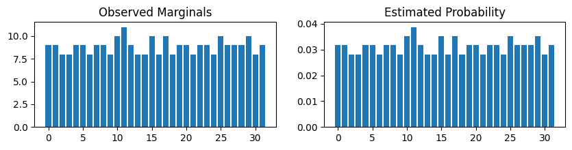
Step 4: View the true marginals against estimated marginals

# Compare a larger clique against the true marginals.
fig, axes = plt.subplots(nrows=1, ncols=2, figsize=(10, 2))
visitorTeamAbbr_marginal = observed_factor_dict[("visitorTeamAbbr",)]
total_states = np.prod(visitorTeamAbbr_marginal.cardinality)
axes[0].bar(
    range(total_states),
    visitorTeamAbbr_marginal.values.flatten(),
)
axes[0].set_title("Observed Marginals")
axes[1].bar(
    range(total_states),
    modeled_factor.marginalize(
        ["homeTeamAbbr", "homeWin"], inplace=False
    ).values.flatten(),
)
axes[1].set_title("Estimated Probability")
plt.show()

Modeling the home & visitor scores

Now, we add back in the score for the home and visitor teams.

Step 1: Make a new df from games with the score columns

COLUMNS_2 = ["homeTeamAbbr", "visitorTeamAbbr", "homeFinalScore", "visitorFinalScore"]
df2 = games[COLUMNS_2]
df2.head()

	homeTeamAbbr	visitorTeamAbbr	homeFinalScore	visitorFinalScore
0	NYG	DAL	0	40
1	NYJ	BUF	22	16
2	NE	PHI	20	25
3	BAL	HOU	25	9
4	MIN	TB	17	20

# This time, more marginals are possible.
marginals_2 = list(
    itertools.chain.from_iterable(
        [list(itertools.combinations(COLUMNS_2, i)) for i in range(1, 5)]
    )
)
marginals_2

[('homeTeamAbbr',),
 ('visitorTeamAbbr',),
 ('homeFinalScore',),
 ('visitorFinalScore',),
 ('homeTeamAbbr', 'visitorTeamAbbr'),
 ('homeTeamAbbr', 'homeFinalScore'),
 ('homeTeamAbbr', 'visitorFinalScore'),
 ('visitorTeamAbbr', 'homeFinalScore'),
 ('visitorTeamAbbr', 'visitorFinalScore'),
 ('homeFinalScore', 'visitorFinalScore'),
 ('homeTeamAbbr', 'visitorTeamAbbr', 'homeFinalScore'),
 ('homeTeamAbbr', 'visitorTeamAbbr', 'visitorFinalScore'),
 ('homeTeamAbbr', 'homeFinalScore', 'visitorFinalScore'),
 ('visitorTeamAbbr', 'homeFinalScore', 'visitorFinalScore'),
 ('homeTeamAbbr', 'visitorTeamAbbr', 'homeFinalScore', 'visitorFinalScore')]

Step 2: Junction Tree creation directly from the data’s marginals

# Instead of creating our graph from every possible combination, we can build
# directly from the dataframe, and then setting each factor equal to 0.0.
G_2 = JunctionTree()
nodes = COLUMNS_2
observed_factor_dict = FactorDict.from_dataframe(
    games,
    marginals=marginals_2,
)
factors_2 = observed_factor_dict = [
    i.identity_factor() for i in observed_factor_dict.values()
]
G_2.add_node(node=COLUMNS_2)
G_2.add_factors(factors_2[-1])
G_2.check_model()

True

# We have a single clique, including all of the dataframe's columns.
print(G_2.nodes)
print(G_2.factors)

[('homeTeamAbbr', 'visitorTeamAbbr', 'homeFinalScore', 'visitorFinalScore')]
[<DiscreteFactor representing phi(homeTeamAbbr:32, visitorTeamAbbr:32, homeFinalScore:45, visitorFinalScore:40) at 0x1683479d0>]

Step 3: Use MirrorDescentEstimator to fit a JunctionTree to the data’s marginals

# Initialize the new estimation.
estimator_2 = MirrorDescentEstimator(model=G_2, data=games)

INFO:pgmpy: Datatype (N=numerical, C=Categorical Unordered, O=Categorical Ordered) inferred from data: 
 {'Unnamed: 0': 'N', 'season_type': 'N', 'week': 'N', 'homeTeamAbbr': 'C', 'homeFinalScore': 'N', 'visitorTeamAbbr': 'C', 'visitorFinalScore': 'N', 'homeWin': 'C'}

%%time
_ = estimator_2.estimate(
    marginals=marginals_2, metric="L2", iterations=600
)

  0%|          | 0/600 [00:00<?, ?it/s]


CPU times: user 1min 24s, sys: 1min 40s, total: 3min 4s
Wall time: 3min 8s

tree_2 = estimator_2.belief_propagation.junction_tree
modeled_factor_2 = tree_2.factors[0]

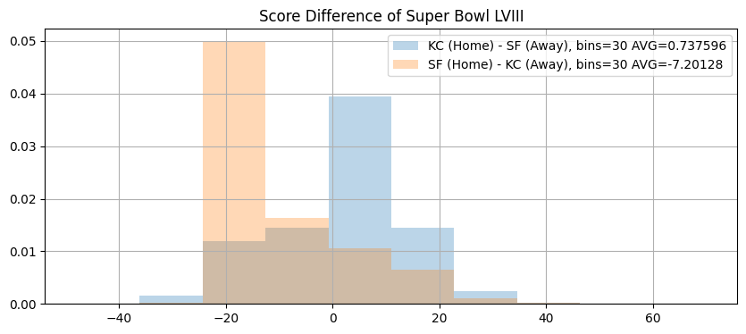
Step 4: Perform a query on a future game

# Inference for a hypothetical game.
sf_kc = BeliefPropagation(tree_2).query(
    variables=["homeFinalScore", "visitorFinalScore"],
    evidence={"homeTeamAbbr": "KC", "visitorTeamAbbr": "SF"},
    joint=True,
    show_progress=True,
)
kc_sf = BeliefPropagation(tree_2).query(
    variables=["homeFinalScore", "visitorFinalScore"],
    evidence={"homeTeamAbbr": "SF", "visitorTeamAbbr": "KC"},
    joint=True,
    show_progress=True,
)

assert isinstance(sf_kc, DiscreteFactor)
sf_kc_sample = sf_kc.sample(1_000_000)
assert isinstance(kc_sf, DiscreteFactor)
kc_sf_sample = kc_sf.sample(1_000_000)

plt.figure(figsize=(10, 4))
sf_kc_diff = sf_kc_sample.homeFinalScore - sf_kc_sample.visitorFinalScore
sf_kc_diff.hist(
    alpha=0.3,
    label=f"KC (Home) - SF (Away), bins=30 AVG={sf_kc_diff.mean()}",
    density=True,
)
kc_sf_diff = kc_sf_sample.homeFinalScore - kc_sf_sample.visitorFinalScore
kc_sf_diff.hist(
    alpha=0.3,
    label=f"SF (Home) - KC (Away), bins=30 AVG={kc_sf_diff.mean()}",
    density=True,
)
plt.title("Score Difference of Super Bowl LVIII")
plt.legend()
plt.show()