Ising Model (Theory, pt. 1)
A post about the theory of the Ising Model.
Ising Model
I have talked before about Lagrangians and Hamiltonians for classical systems, now it is time to see one from statistical physics. Before getting into the code, lets setup some terminology and definitions.
I followed Chapter 31 of MacKay’s Information Theory, Inference, and Learning Algorithms which covers Ising Models in great detail. I followed up on Wikipedia for some omitted details.
Ising Model Setup
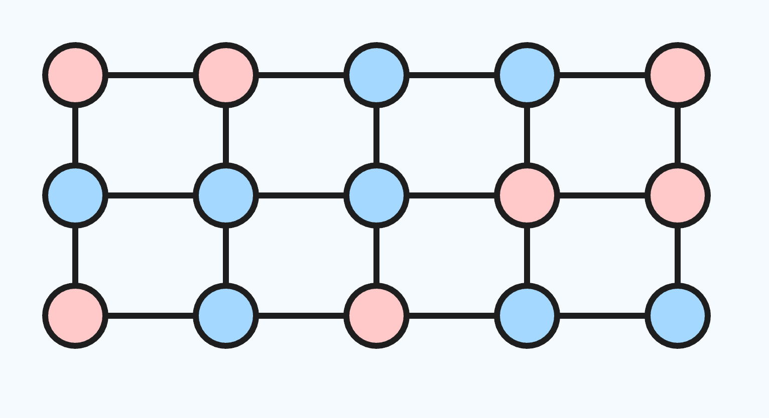
Consider a set of variables
\[x_k \in \{ -1, +1 \}\]over
\[G \in \{ -1, +1 \}^{(N \times M)}\]a $(N \times M)$ dimensional lattice. The states $-1$ and $+1$ of $x_k$ represent the spins of atoms. For neighboring $(x_n, x_m)$ pairs, we define $J_{n, m}$ to be an interaction variable describing the affinity of $(x_n, x_m)$. We have two cases for $J_{n, m}$:
- $\pmb{J_{n, m} > 0}$ will give $(x_n, x_m)$ positive affinity leading towards a ferromagnetic system.
- $\pmb{J_{n, m} < 0}$ will give $(x_n, x_m)$ negative affinity leading towards an antiferromagnetic system
Lastly, we define $h$ as a (constant for now) applied magnetic field on each individual atom, $x_k$. $h$ is an individual bias for each $x_k$ that encourages each atom to favor a particular state ($-1$ or $+1$).
Ising Hamiltonian
Now we are ready to define the Hamiltonian. It will consist of two potential energies, one for all pairs of $(x_n, x_m)$ representing the energy created from each individual atom’s magnetic dipole and the other for all $x_n$ representing how the applied magnetic field affects the lattice as a whole:
\[H(x; J, h) = -\frac{1}{2}\sum_{n, m}J_{n, m}x_nx_m - \sum_n h x_n\]A factor of $\frac{1}{2}$ is used so that we do not double count pairs as we iterate over $(x_n, x_m)$ and $(x_m, x_n)$, and a negative is taken by convention. Previously, we had momentum ($p$) terms in the Hamiltonian giving the Kinetic energy of the system. Since these atoms are assumed to be locked in a static lattice, only their positions $x_n$ contribute towards the total energy.
Boltzmann Distribution
The probability of any specific configuration of atoms is given by the Boltzmann distribution:
\[P_\beta(x) = \frac{\exp{-\beta H(x; J, H)}}{Z_\beta} = \frac{\exp{-\beta H(x; J, H)}}{\sum_x \exp{-\beta H(x; J, H)}}\]Where $\beta = \frac{1}{k_B T}$ with $k_B$ being Boltzmann’s constant and $T$ the temperature. Importantly, the partition function is described as:
\[Z_\beta = \sum_x \exp{-\beta H(x; J, H)}\]For a specific instantiation of $G$, we can read off each state of $x_n$ giving us a vector $x$. The probability we will remain in this state $x$ (in the long term), will be the ratio of $\exp{-\beta H(x; J, H)}$ normalized by every other possible configuration (i.e. $Z_\beta$). There will be $2 ^ {N \times M}$ of these configurations in total, making $P_\beta(x)$ exponential to compute without approximate inference.
Connection to Machine Learning
The Boltzmann distribution is also used in Machine Learning under the name Boltzmann machines which uses a similar energy to $H$ except $h$ is allowed to vary with each index $n$:
\[E = -\sum_{n < m}w_{n, m}x_nx_m - \sum_n \theta_n x_n\]Boltzmann Machines gave rise to Restricted Boltzmann Machines (RBM) and Deep Boltzmann Machines (DBM) which were the first examples of “fully connected networks” now commonly seen in Neural Networks. All of these models are special cases of the Markov Random Field which is an undirected probabilistic graphical model. See Box 4.C on page 126 of the Koller & Friedman Textbook.
Statistical Physics of the Ising Model
With a probability distribution specified, it is now possible to define statistical quantities of the Ising Model system. Depending on your background, some of these terms will be more familiar than others. Since I am more familiar with statistics, I will start from that perspective and mention the connections to thermodynamics and information theory. First, we can define the expected energy of the Ising Model:
\[\begin{flalign*} \mathbb E_{x \sim P_\beta(x)}[H(x)] &= \sum_x P_\beta(x) H(x) \\ &= \sum_x \frac{\exp{-\beta H(x)}}{Z_\beta} H(x) \\ &= \frac{1}{Z_\beta} \sum_x H(x)\exp{[-\beta H(x)]} \\ &= \bar H \\ &= -\frac{\partial \ln Z_\beta}{\partial \beta} \end{flalign*}\]We can connect $\bar H$ to heat capacity from thermodynamics as:
\[C := \frac{\partial}{\partial T} \bar H\]To compute the variance of $H(x)$, it is easier to start from $\frac{\partial \ln Z_\beta}{\partial \beta} = -\bar H$ and differentiate a second time wrt $\beta$:
\[\begin{flalign*} \frac{\partial}{\partial \beta}\frac{\partial \ln Z_\beta}{\partial \beta} &= \frac{\partial}{\partial \beta} (\frac{1}{Z_\beta} \sum_x -H(x)\exp{[-\beta H(x)]}) \\ &=(\frac{\partial}{\partial \beta}\frac{1}{Z_\beta})\cdot \sum_x -H(x)\exp{[-\beta H(x)]} + \frac{1}{Z_\beta} \cdot (\frac{\partial}{\partial \beta} \sum_x -H(x)\exp{[-\beta H(x)]}) \\ &= -(\frac{1}{Z_\beta})^2(\sum_x -H(x)\exp{[-\beta H(x)]})^2 + \frac{1}{Z_\beta}\sum_x H(x)^2\exp{[-\beta H(x)]} \\ &= -(\frac{1}{Z_\beta}\sum_x H(x)\exp{[-\beta H(x)]})^2 + \frac{1}{Z_\beta}\sum_x H(x)^2\exp{[-\beta H(x)]} \\ &= -\bar H(x) ^2 + \frac{1}{Z_\beta}\sum_x H(x)^2\exp{[-\beta H(x)]} \\ &= \frac{1}{Z_\beta} \sum_x \big(H(x)^2\exp{[-\beta H(x)]}\big) - \bar H(x)^2 \\ &= \mathbb E_{x \sim P_\beta(x)}[H(x)^2] - \bar H(x)^2 \\ &= \mathbb V[H(x)] \end{flalign*}\]And putting it all together shows a relationship between $\mathbb V[H(x)]$ and $C$:
\[\begin{gather*} \frac{\partial \bar H(x)}{\partial T} = -\frac{\partial}{\partial T}\frac{\partial \ln Z_\beta}{\partial \beta} \\ = -\frac{\partial}{\partial T}\frac{\partial \ln Z_\beta}{\partial \beta} (\frac{\partial T}{\partial \beta} \frac{\partial \beta}{\partial T}) \\ = -\frac{\partial^2 \ln Z_\beta}{\partial \beta^2}\frac{\partial \beta}{\partial T} \\ = -\mathbb V[H(x)](-\frac{1}{k_B T^2}) \\ \therefore C = \frac{\mathbb V[H(x)]}{k_B T^2} = k_B\beta^2 \cdot \mathbb V[H(x)] \end{gather*}\]Which means that the variance (over the states) of the system is proportional to the system’s heat capacity. And lastly, we can make a connection to entropy from information theory:
\[\begin{flalign*} \mathbb E_{x \sim P_\beta(x)}[-\ln P_\beta(x)] &= \sum_x - P_\beta(x) \ln P_\beta(x) \\ &= \sum_x -\frac{\exp{-\beta H(x)}}{Z_\beta} \cdot \ln {\frac{\exp{-\beta H(x)}}{Z_\beta}} \\ &= \sum_x-\frac{\exp{-\beta H(x)}}{Z_\beta} (-\beta H(x) - \ln{Z_\beta}) \\ &= \sum_x \beta\frac{H(x)\exp{-\beta H(x)}}{Z_\beta} + \frac{\ln{Z_\beta}\exp{-\beta H(x)}}{Z_\beta} \\ &= \beta \bar H(x) + \frac{\ln{Z_\beta}}{Z_\beta}\sum_x \exp{-\beta H(x)} \\ &= \beta \bar H(x) + \ln{Z_\beta} \frac{Z_\beta}{Z_\beta} \\ &= \beta \bar H(x) + \ln{Z_\beta} \end{flalign*}\]Arriving at $\frac{\partial \ln Z_\beta}{\partial \beta} = -\mathbb E_{x \sim P_\beta(x)}[H(x)]$ and $\frac{\partial^2 \ln Z_\beta}{\partial \beta^2} = \mathbb V[H(x)]$ should not be surprising considering $P_\beta(x) = \frac{\exp{-\beta H(x; J, H)}}{Z_\beta}$ is a member of the exponential family with sufficient statistic $T(x) = H(x; J, H)$ and partition function $Z_\beta$.
Approximate Inference
From the above calculations, we see the importance of $Z_\beta$. There are many ways to simplify the inference problem so that computing $P_\beta(x)$ (and $Z_\beta$ by extension) does not actually take exponential time. The main categories of doing this are:
- Sampling-based Inference includes Markov Chain Monte Carlo (MCMC) algorithms. Variants include Metropolis Hastings (MH) & Gibbs Sampling (a special case of Metropolis-Hastings), also known as Glauber Dynamics.
- Variational Inference includes Mean Field Inference and Loopy Belief Propagation. See Box 11.C on page 409 of the Koller & Friedman Textbook for more details on Loopy Belief Propagation applied to the Ising Model.
For the rest of this post, I will focus on the former case, Sampling-based Inference. I will borrow the notation from the CS228 course notes.
Algorithm Sketch
First, we give the pseudo code of how MCMC on the Ising Model works:
1
2
3
4
1. Choose an atom, x_{n, m}.
2. Compute a difference in energy, delta_H, if the atom were to change spins.
3. Flip the spin with probability based on delta_H.
4. Repeat the above steps N Times.
The differences are primarily in step 1) how to select an atom each iteration and 3) the probability of flipping the spin.
Metropolis Hastings
For MH algorithm, one possible transition matrix is moving uniformly across atoms \(n \sim U\{1..., NM\}\) and setting $x_n$ to $-x_n$ (leaving the remaining $x_{-n}$ unchanged). We can express this in vector form as $x’ = [x_1, …, -x_n, … x_{N \times M}]$ and $x = [x_1, …, x_n, … x_{N \times M}]$ making the transition kernel:
\[Q(x' | x) = Q(x | x') = \frac{1}{NM}\]The acceptance probability would then be:
\[A(x' | x) = \min{\big[ 1, \frac{P(x')Q(x | x')}{P(x)Q(x' | x)} \big ]} = \min{\big[ 1, \frac{P(x')}{P(x)} \big ]} = \min{\big[ 1, \exp{-\beta (H(x') - H(x))} \big ]}\]Importantly, cancelling out $Q(x’ | x)$, $Q(x | x’)$, and $Z_\beta$. Recognizing that $x’$ and $x$ differ only at atom $n$, we can make two simplifications:
- Note that $H(x’) - H(x)$ will only differ in the $(i, j)$ pairs involving $i = n$. Thus, we can only focus on that summand in $H$.
- Since we are only considering a single summand, we can drop the leading $\frac{1}{2}$ since that was only accounting for double counting each $(i, j)$ and $(j, i)$ pair.
Making the final acceptance probability:
\[A(x' | x) = \min{\big[ 1, \exp{-2\beta x_n \sum_m J_{n,m} x_m + h} \big ]}\]Which matches the equation found in 31.1 of Information Theory, Inference, and Learning Algorithms on page 402. It is typical to loop through the atoms from left to right, top to bottom when applying MH updates.
Gibbs Sampling
As a special case of MH, we sample in a coordinate-wise fashion using the conditional distribution:
\[P(x_n | \{x_i\}_{i \neq n})\]Selecting $n$ randomly from all of the atoms each iteration. If MH is gradient descent, then Gibbs Sampling is coordinate descent. Except of course instead of optimization, we are performing MCMC steps. We can compute the acceptance probability for Gibbs sampling:
\[A(x' | x) = \min{\big[ 1, \frac{P(x')Q(x | x')}{P(x)Q(x' | x)} \big ]} = \min{\big[ 1, \frac{P(x_n')Q(x_n | x_n')}{P(x_n)Q(x_n' | x_n)} \big ]}\]Since only one coordinate changes in each Markov Chain step. And in particular,
\[Q(x_n | x_n') = P(x_n | \{x_i\}_{i \neq n})\] \[Q(x_n' | x_n) = P(x_n' | \{x_i\}_{i \neq n})\]Making,
\[\frac{P(x_n')Q(x_n | x_n')}{P(x_n)Q(x_n' | x_n)} = \frac{\frac{P(x_n')P(x_n)}{P(\{x_i\}_{i \neq n})}}{\frac{P(x_n)P(x_n')}{P(\{x_i\}_{i \neq n})}} = 1\]And the overall acceptance probability also 1, meaning we always accept the proposal step. That is to say, Gibbs Sampling is directly sampling from the conditional distribution each step. To compute this, we need:
\[\begin{flalign*} P(x_n = 1 | \{x_i\}_{i \neq n}) &= \frac{P(x_n = 1 \bigcap \{x_i\}_{i \neq n} )}{P(\{x_i\}_{i \neq n})} \\ &= \frac{P(x_n = 1 \bigcap \{x_i\}_{i \neq n} )}{P(x_n = 1 \bigcap \{x_i\}_{i \neq n} ) + P(x_n = -1 \bigcap \{x_i\}_{i \neq n})} \end{flalign*}\]For ease of notation, define:
\[P(x_n = 1 \bigcap \{x_i\}_{i \neq n} ) = P(x_n^+)\]and similarly for $P(x_n^-)$. Then,
\[P(x_n = 1 | \{x_i\}_{i \neq n}) = \frac{P(x_n^+)}{P(x_n^+) + P(x_n^-)}\]Let $p = \frac{P(x_n^+)}{P(x_n^-)}$, then:
\[\begin{flalign*} P(x_n = 1 | \{x_i\}_{i \neq n}) &= \frac{pP(x_n^-)}{pP(x_n^-) + P(x_n^-)} \\ &= \frac{p}{1 + p} \\ &= \frac{\exp \ln p}{1 + \exp \ln p} \\ &= \sigma(\ln p) \end{flalign*}\]Where $\sigma$ is the sigmoid function. Applying $\sigma$ in this way is common in Machine Learning derivations and $\ln p$ is similar to the log-odds. To compute this quantity we need:
\[\begin{flalign*} \ln p &= \ln \frac{P(x_n^+)}{P(x_n^-)} \\ &= \ln \big (\frac{\exp -\beta H(x_n^+)}{\exp -\beta H(x_n^-)} \cdot \frac{Z_\beta}{Z_\beta} \big ) \\ &= -\beta (H(x_n^+) - H(x_n^-)) \end{flalign*}\]Which now requires our original definition of $H$ and some record keeping. We only need to consider atom $n$ giving the same two simplifications from the MH algorithm:
\[\begin{flalign*} H(x_n^+) - H(x_n^-) &= -\sum_{m}J_{n, m}(1)x_m - h (1) - (-\sum_{m}J_{n, m}(-1)x_m - h (-1)) \\ &= -\sum_{m}J_{n, m}x_m - h - \sum_{m}J_{n, m}x_m - h \\ &= -2(\sum_{m}J_{n, m}x_m + h) \end{flalign*}\]Putting things together gives us a concrete conditional probability we can sample from:
\[P(x_n = 1 | \{x_i\}_{i \neq n}) = \sigma(2\beta\sum_{m}J_{n, m}x_m + h)\]Which matches the expression found in 31.1 of Information Theory, Inference, and Learning Algorithms on page 402. Also, see this related blog post by LeftAsExercise for another excellent presentation of this derivation.
Summary
In this post I discussed the Ising Model, its connections to Machine Learning, and its statistical properties. I then derived two approximate inference algorithms, Metropolis Hastings and Gibbs Sampling. In the second part of this post, I will convert the theory to code.