Ising Model (Computation, pt. 2)

A post about the computation of the Ising Model.

Ising Model Code

Code inspired by this post by @Jake VanderPlas which compares Python against cPython.

import numpy as np
import pandas as pd
import plotly.express as px
import plotly.graph_objects as go
from IPython.display import display, Markdown
from typing import List

np.random.seed(1)

MCMC Implementations

Below I copy+pasted the functions directly from @Jake VanderPlas blog post. Looking back to the update equations for MH, MCMC:

\[A(x' | x) = \min{\big[ 1, \exp{-2\beta x_n \sum_m J_{n,m} x_m + h} \big ]}\]

We recognize the original blog post’s update as a MH, MCMC step.

# Functions from Jake VanderPlas's blog post.
def random_spin_field(N, M):
    return np.random.choice([-1, 1], size=(N, M))


# Add an `update_fn` arg.
def ising_step(field, update_fn, beta=0.4):
    N, M = field.shape
    for n_offset in range(2):
        for m_offset in range(2):
            for n in range(n_offset, N, 2):
                for m in range(m_offset, M, 2):
                    update_fn(field, n, m, beta)
    return field


def _ising_update(field, n, m, beta):
    total = 0
    N, M = field.shape
    for i in range(n - 1, n + 2):
        for j in range(m - 1, m + 2):
            if i == n and j == m:
                continue
            total += field[i % N, j % M]
    dE = 2 * field[n, m] * total
    if dE <= 0:
        field[n, m] *= -1
    elif np.exp(-dE * beta) > np.random.rand():
        field[n, m] *= -1

We can also add in the Gibbs Sampling step:

\[P(x_n = 1 | \{x_i\}_{i \neq n}) = \sigma(2\beta\sum_{m}J_{n, m}x_m + h)\]

# Also make a random stepping Ising update.
def sigmoid(x: float) -> float:
    # 700 seems to be the magic number where numpy will overflow.
    # In this case, analytically handle the probability
    if -x > 700:
        return 0.0
    return float(1 / (1 + np.exp(-x)))


def _ising_update_gibbs(field: np.ndarray, n: int, m: int, beta: float) -> None:
    total = 0
    N, M = field.shape
    for i in range(n - 1, n + 2):
        for j in range(m - 1, m + 2):
            if i == n and j == m:
                continue
            total += field[i % N, j % M]
    dE = 2 * beta * total
    if sigmoid(dE) > np.random.rand():
        field[n, m] = 1
    else:
        field[n, m] = -1

Plotting Helpers

A couple helper functions so that we can plot to markdown.

# Plotting helper functions.
def render_plotly_html(fig: go.Figure) -> None:
    """Display a Plotly figure in markdown with HTML."""
    # Ensure frame is square
    display(
        Markdown(
            fig.to_html(
                include_plotlyjs="cdn",
            )
        )
    )


def _grid_to_long(grid: np.ndarray) -> np.ndarray:
    """Convert a N x M matrix into a (N x M, 2) long vector."""
    # x coordinate, y coordinate, spin of the coordinate.
    return np.vstack(
        [*map(lambda x: x.flatten(), np.indices(grid.shape)), grid.flatten()]
    ).T


def grids_to_long(grids: List[np.ndarray]) -> pd.DataFrame:
    """Convert a n-list of grid matrices into a long-format DataFrame.

    Args:
        grids: List of grid matrices ordered by time.

    Returns:
        DataFrame with each N x M matrix converted to a (N x M, 2) section.
        Each section is indexed by the order in `grids`.
    """
    t = np.array([[i] * np.prod(grid.shape) for i, grid in enumerate(grids)])
    df = pd.DataFrame(np.concatenate([_grid_to_long(i) for i in grids]))
    df["t"] = t.flatten()
    df.columns = ["x", "y", "spin", "t"]
    return df

Sampling

Now we can sample both MH MCMC and Gibbs Sampling and compare the results.

N, M = 40, 40
STEPS = 500
BETA = 0.25
# Start from the same random initial configuration.
images = [random_spin_field(N, M)]

mh_images = images.copy()
for i in range(STEPS):
    mh_images.append(ising_step(mh_images[-1].copy(), beta=BETA, update_fn=_ising_update))
mh_steps = grids_to_long(mh_images)
mh_steps["sampler"] = "MH"

gibbs_images = images.copy()
for i in range(STEPS):
    gibbs_images.append(ising_step(gibbs_images[-1].copy(), beta=BETA, update_fn=_ising_update_gibbs))
gibbs_steps = grids_to_long(gibbs_images)
gibbs_steps["sampler"] = "Gibbs"

Plots

# Plot the simulation as a time lapse in Plotly.
fig = px.scatter(
    mh_steps,
    x="x",
    y="y",
    color="spin",
    color_continuous_scale="thermal",
    animation_frame="t",
    hover_name="t",
)
fig.update(layout_coloraxis_showscale=False)
# Ensure frame is square
fig.update_yaxes(
    scaleanchor="x",
    scaleratio=1,
)
render_plotly_html(fig)

fig.show()

# Plot the simulation as a time lapse in Plotly.
fig = px.scatter(
    gibbs_steps,
    x="x",
    y="y",
    color="spin",
    color_continuous_scale="thermal",
    animation_frame="t",
    hover_name="t",
)
fig.update(layout_coloraxis_showscale=False)
# Ensure frame is square
fig.update_yaxes(
    scaleanchor="x",
    scaleratio=1,
)
render_plotly_html(fig)

fig.show()

Analysis

Magnetism

For magnetism, we are interested in:

\[m = \frac{1}{N}\sum_n x_n\]

This is simply a groupby on our datasets.

average_magnetism = (
    pd.concat([mh_steps, gibbs_steps])
    .groupby(["sampler", "t"])
    .spin.mean()
    .reset_index()
)

magnetism = px.line(
    average_magnetism, x="t", y="spin", color="sampler", title="Average Magnetism"
)
render_plotly_html(magnetism)

magnetism.show()

magnetism_hist = px.histogram(
    average_magnetism, x="spin", color="sampler", title="Average Magnetism Distribution", opacity=0.7
)
render_plotly_html(magnetism_hist)

magnetism_hist.show()

magnetism_std = px.line(
    pd.concat([mh_steps, gibbs_steps])
    .groupby(["sampler", "t"])
    .spin.std()
    .reset_index(),
    x="t",
    y="spin",
    color="sampler",
    title="Magnetism Std Dev"
)
render_plotly_html(magnetism_std)

magnetism_std.show()

The average magnetism and std dev of magnetism are comparable, with Gibbs Sampling having slower convergence.

Energy

Recalling our Hamiltonian from the Ising Model from before:

\[H(x; J, h) = -\frac{1}{2}\sum_{n, m}J_{n, m}x_nx_m - \sum_n h x_n\]

def energy(field: np.ndarray) -> np.ndarray:
    N, M = field.shape
    energies = np.zeros_like(field)
    for n in range(N):
        for m in range(M):
            energy_position(energies, field, n, m)
    return energies


def energy_position(energies: np.ndarray, field: np.ndarray, n: int, m: int) -> None:
    total = 0
    N, M = field.shape
    for i in range(n - 1, n + 2):
        for j in range(m - 1, m + 2):
            if i == n and j == m:
                continue
            total += field[n, m] * field[i % N, j % M]
    energies[n, m] = -0.5 * total

mh_energies = np.array(list(map(energy, mh_images)))
gibbs_energies = np.array(list(map(energy, gibbs_images)))

t = list(range(len(mh_images)))
energies = pd.DataFrame(
    {
        "t": t + t,
        "sampler": ["MH"] * len(mh_images) + ["Gibbs"] * len(gibbs_images),
        "energy": np.vstack(
            [mh_energies.mean((1, 2)), gibbs_energies.mean((1, 2))]
        ).flatten(),
        "std_energy": np.vstack(
            [mh_energies.std((1, 2)), gibbs_energies.std((1, 2))]
        ).flatten(),
    }
)

energies_fig = px.line(
    energies,
    x="t",
    y="energy",
    color="sampler",
    title="Average Energy"
)
render_plotly_html(energies_fig)

energies_fig.show()

energy_hist = px.histogram(
    energies, x="energy", color="sampler", title="Average Energy Distribution", opacity=0.7
)
render_plotly_html(energy_hist)

energy_hist.show()

energies_std = px.line(
    energies, x="t", y="std_energy", color="sampler", title="Std Dev Energy"
)
render_plotly_html(energies_std)

energies_std.show()

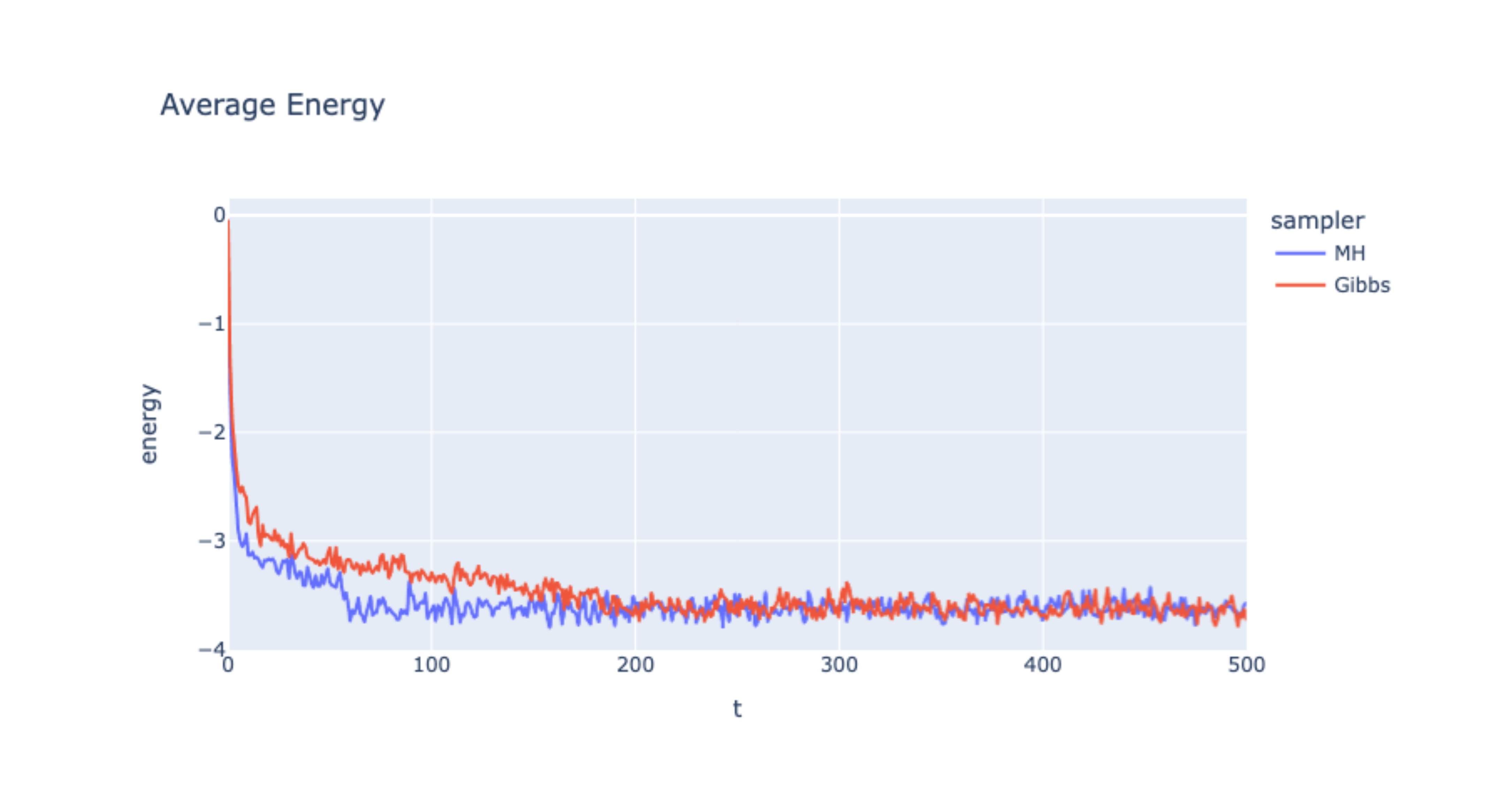
Energy is also pretty comparable, again, with Gibbs having slower convergence.

Summary

Instead of evaluating the partition function $Z_\beta$ directly, we can estimate some of the statistical properties with MCMC samples. Its interesting to me that despite the MH and Gibbs simulations looking quite different the average and variability of the energy and magnetism seem to converge to the same value. This indicates that both MH and Gibbs are sampling from the same long term distribution.

# A little magic to automatically write my blog :)
import subprocess

subprocess.run(["jupyter", "nbconvert", "--to", "markdown", "ising_model.ipynb"])