Interval Detector

You have a statistical detector capable of raising alerts on time series data (i.e. number of crashes in an hour or average bandwidth for a fleet of servers) and received a question from the engineering team:

Q: How many alerts should we wait for before actually “alerting” the oncall?

A: You’ve been waiting to send the alerts???

A detection that is consistently passing some threshold should receive more weight than a spurious detection. But since the critical value of a Statistical Test is carefully calibrated for just a single test, we need to ensure the probability of raising a false positive (i.e. Type-I Error) does not exceed a certain threshold when considering multiple rejections.

Just Show Me The Code…

Check out this code to see a working implementation.

If you are curious about the statistical formalisms; then read on 😀

FWER and Bonferroni Corrections

Before diving into the solution, let’s formalize the problem and consider a simple solution.

The Problem

Consider a distribution that has a time-dependent parameter \(\mathcal D(\mu_t)\) for \(t=1,...,T\). The granularity of \(\mu_t\) will depend on an aggregation scheme (i.e. hourly, daily, weekly) which is determined by the use case. Now, instead of a single $H_0$ vs. $H_a$ comparison, we will consider a family of level-$\alpha$ tests, $H_F={H_1, …, H_T}$ which can be used to make inferences on $\mu_t$ simultaneously. The Type-I Error for this family-wise test is generalized to a Family-wise Error Rate (FWER) for $\bigcup_{i=1}^T H_i$:

\[\begin{flalign*} FWER &= P(\text{Single rejection in } \bigcup_{i=1}^T H_i | H_F \text{ all true}) \\ &= P(\text{Rejecting at least one } H_i | H_F \text{ all true}) \\ &= 1 - P(\text{No rejections }| H_F \text{ all true}) \label{eq:FWER} \end{flalign*}\]

Consider a numerical example with \(T \geq 14\) and \(\alpha=0.05\) of a naive test which illustrates a major shortcoming called Multiple Comparisons. We have,

\[\begin{equation*} FWER \geq 1 - (1 - \alpha)^T = 1 - 0.95^{14} \approx 0.512 \end{equation*}\]

Which will commit a Type-I error more than half of the time. This shows the fundamental problem of Multiple Comparisons or Multiple Testing, if \(\alpha\) (or another part of the test criterion) is not adjusted for \(T\) simultaneous comparisons, then the resulting \(FWER\) can be significantly inflated.

The Solution

A popular way to fix this is known as Bonferroni Correction, which is an application of Boole’s Inequality:

\[\begin{equation*} \alpha' = \frac{\alpha}{T} \label{eqn:bonferroni_correction} \end{equation*}\]

Then, the correction above becomes:

\[\begin{equation*} FWER = 1 - (1 - \alpha')^T = 1 - (1 - 0.05 / 14)^{14} \approx 0.048 \end{equation*}\]

Which has successfully corrected \(FWER \leq \alpha\). While this approach certainly works, we have disregarded the ordering of the data (\(t=1,...,T\)) and treated the tests as iid.

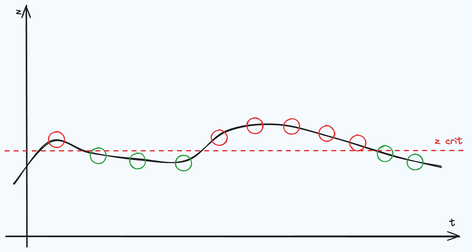
Interval Detections

So how do we include the ordering of the tests into the FWER calculation? We want a test that says simultaneously rejecting \(\{H_i, ..., H_{i + d - 1}\}\) for some \(d \geq 1\), provides more information than rejecting \(H_i\) and \(H_j\) where \(|i - j| > d\). First, define a function that serves as an indicator function of whether \(d\) rejections has occurred in \(d\) timestamps,

\[\begin{equation*} f(i, d) = \begin{cases} 1 \quad \text{if $\displaystyle\sum_{k=i}^{i+d-1} \mathbb I\{H_i \text{ rejects}\} = d$} \\ 0 \quad \text{otherwise} \end{cases} \label{eqn:sliding_window} \end{equation*}\]

And apply a sliding window operation across the timestamps to compute the test statistic:

\[V(d) = \sum_{i=1}^{T- d +1} f(i, d)\]

Which computes the number of times we had a window of \(d\) sequential rejections in our time series. With this sliding window test statistic, define the Hypothesis Test:

\[\begin{equation*} H_0: V(d) = 0 \quad vs. \quad H_a: V(d) \geq 1 \end{equation*}\]

Which has FWER of,

\[\begin{equation} FWER = P(V(d) \geq 1 | H_F \text{ all true}) \label{eqn:fwer_interval_general} \end{equation}\]

Whew! We have our test. Now, we just have to work out the sampling distribution of \(V(d)\) to turn this statistical test into a numerical computation.

FWER Under Independence

As a first approach to computing FWER, lets reason about the sampling distribution with an independence assumption:

\[\begin{equation} P(H_i \text{ and } H_j \text{ rejects}) = P(H_i \text{ rejects}) \cdot P(H_j \text{ rejects}) \forall i \neq j \label{eqn:independence} \end{equation}\]

Where each individual \(H_i\) is just a biased coin flip,

\[P(H_i \text{ rejects}) \stackrel{iid}{\sim} Bernoulli(p=\alpha)\]

Okay, what are the implications of this in terms of \(\eqref{eqn:fwer_interval_general}\)? We can write,

\[\begin{gather*} FWER = P(V(d) \geq 1 | H_F \text{ all true} \cap H_i \perp H_j: i\neq j) \\ = P(\text{At least 1 run of $d$ consecutive biased coin flips}) \end{gather*}\]

Which makes sense, we are interested when we have at least one run of \(d\) rejections. Luckily, we can use a recursive relation to solve this in \(O(T)\) time. Define \(r_j^{(d, p)}\) to be the event that at least 1 run of \(d\), probability \(p\) successes exists up to (and including) the \(j^{th}\) index. Initialize the recursion with \(r_j^{(d, p)}=0\) for \(j=0,...,d-1\) (since its impossible to have \(d\) rejections before \(d\) timestamps have occured). Then:

\[\begin{equation} P(r_j^{(d, p)}) = p^d + \sum_{i=0}^{d-1} p^i \cdot (1-p) \cdot P(r_{j-i-1}^{(d, p)}) \label{eqn:independent_recursion} \end{equation}\]

Finally, iterating \eqref{eqn:independent_recursion} for $T-d+1$ iterations, we arrive at:

\[\begin{equation} FWER = P(r_{T}^{(d, \alpha)}) \end{equation}\]

Seeing the recursive relation \eqref{eqn:independent_recursion} as repeating a linear combination of the previous $P(r_j^{(d, \alpha)})$ states, we can efficiently implement this recursion with optimized linear algebra packages!

Computing FWER Under Independence with Matrices

Recognizing $P(r_j^{(d, p)})$ in $\eqref{eqn:independent_recursion}$ as being a linear combination of the $P(r_i^{(d, p)})$ states for $i < j$, we can express this in terms of vector-matrix operations. First define a vector of previous states, $\vec r_{j-1:j-d} \in \mathbb R^{1\times(d+1)}$: $$ \begin{equation*} \vec r_{j-1:j-d} = [P(r_{j-1}^{(d, p)}), P(r_{j-2}^{(d, p)}), ..., P(r_{j-d}^{(d, p)}), 1] \end{equation*} $$ And the weight vector $\vec w \in \mathbb R^{(d+1) \times 1}$ as (for the independent case), $$ \begin{equation*} \vec w = \begin{bmatrix} p^0(1-p) \\ p^1(1-p) \\ \vdots \\ p^{d-1}(1-p) \\ p^d \end{bmatrix} \end{equation*} $$ Then, we can rewrite $\eqref{eqn:independent_recursion}$ as a dot product: $$ \begin{equation*} P(r_j^{(d, p)}) = \vec r_{j-1:j-d} \cdot \vec w \end{equation*} $$ Instead of computing the next state as a scalar quantity, can cycle the "states" of $\vec r_{j-1:j-d}$. We introduce the matrix $\pmb C \in \mathbb R^{(d+1)\times d}$ which will update the vector $\vec r_{j-1:j-d}$ to the next state $\vec r_{j:j-d+1}$: $$ \begin{equation*} \pmb C = \left[\begin{array}{c|c} \\ \pmb I_{(d-1)\times(d-1)} & \vec 0_{(d-1)\times 1} \\ \\ \hline \vec 0_{1\times(d-1)} & 0 \\ \hline \vec 0_{1\times(d-1)} & 1 \end{array}\right] \end{equation*} $$ Which makes a one-step update as, $$ \begin{equation*} \vec r_{j:j-d+1} = \vec r_{j-1:j-d} \cdot [\vec w_{(d+1) \times 1)} | \pmb C_{(d+1)\times d}] \end{equation*} $$ And finally, we can make a $(T-d+1)$-step update to solve for state $T$: $$ \begin{equation*} \vec r_{T:T-d+1} = \vec r_{d-1:0} \cdot [\vec w_{(d+1 \times 1)} | \pmb C_{(d+1)\times d}]^{T-d + 1} \end{equation*} $$ Where $\vec r_{d-1:0}$ is initialized as $[\vec 0_{1\times d}, 1]$.

FWER with Relaxed Independence

In most cases, adding the full independence assumption \eqref{eqn:independence} for all \(i\neq j\) is too restrictive for a Null Hypothesis based upon intervals of rejections. Instead, if we reduce this assumption to:

\[\begin{equation} r_{i}^{(d, p)} \perp H_j, \forall i<j \label{eqn:intervals_indep_future_tests} \end{equation}\]

We can retain the recursive formulation of \(\eqref{eqn:independent_recursion}\), but allow some dependency within each updating step of the recursion. In this case, the recurrence relation becomes:

\[\begin{flalign} \begin{split} & P(r_j^{(d, p)}) = P(H_{j-d+1} \text{ rejects} \cap ... \cap H_{j} \text{ rejects}) \\ & + \sum_{i=0}^{d-1} P(\bigcap_{k=j-i}^{j-1} [H_{k} \text{ rejects}] \cap H_{j} \text{ fails to reject} \cap r_{j-i-1}^{(d, p)}) \end{split} \\ \begin{split} & \stackrel{\perp}{=} P(H_{j-d+1} \text{ rejects} \cap ... \cap H_{j} \text{ rejects}) \\ & + \sum_{i=0}^{d-1} P(\bigcap_{k=j-i}^{j-1} [H_{k} \text{ rejects}] \cap H_{j} \text{ fails to reject}) \cdot P(r_{j-i-1}^{(d, p)}) \end{split} \label{eqn:generic_recursion_independence} \end{flalign}\]

Now, the user is required to specify the dependencies within an interval for all time indices \(\{1,...,T\}\) which, in general, is \(\frac{T(T + 1)}{2}\) parameters. Alternatively, we can hypothesize a more tractable dependence structure that balances this full generality with the usability of the method. These options range from auto-regressive models to Gaussian Processes.

Computing FWER Under Relaxed Independence with Matrices

In the case of dependence, $\vec w$ can be updated with the appropriate joint probability distribution from $\eqref{eqn:generic_recursion_independence}$.

A Simple AR(1) Example of Relaxed Independence

Here is one simple example of estimating dependence. Consider the AR(1) process:

\[\begin{equation*} \begin{split} X_t = \rho X_{t-1} + \epsilon_t, \quad \epsilon_t \sim \mathcal N(0, \sigma^2) \\ \mathbb E[X_t] = 0, \quad Cov(X_t, X_{t'}) = \sigma^2\frac{\rho^{|t - t'|}}{1 - \rho^2} \end{split} \label{eqn:ar_1_process} \end{equation*}\]

Where $\rho \in (-1, 1)$ is a parameter controlling the strength of dependency in the test statistic. Which is nothing but a Gaussian Process with a particular kernel:

\[\begin{equation*} k(\tau) = \sigma^2\frac{\rho^{|\tau|}}{1 - \rho^2} \label{eqn:ar_1_process_kernel} \end{equation*}\]

We can then compute the updating equation of \(\eqref{eqn:generic_recursion_independence}\) with numerical methods like this one.

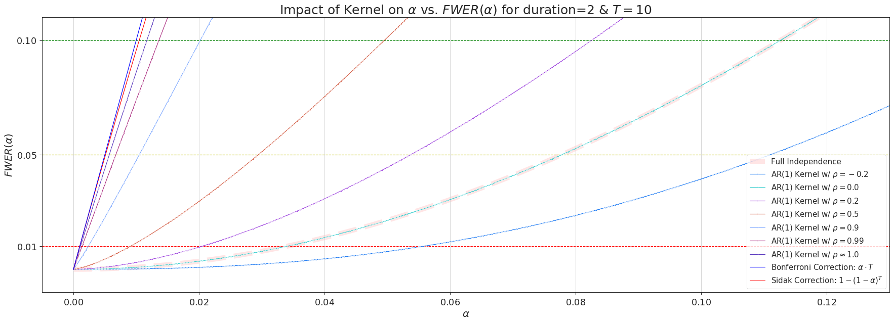
The picture above demonstrates how the choice of $\rho$ impacts $FWER(\alpha)$ in the simple setting of $d=2$ and $T=10$. Specifically, setting $\rho = 0$ will revert \(\eqref{eqn:generic_recursion_independence}\) back to the full independence case of \(\eqref{eqn:independent_recursion}\), \(\rho > 0\) will give more conservative corrections than \(\rho = 0\), but less stringent than the Bonferroni correction.

Summary

In this post, I showed how a Hypothesis Test can be devised to account for the sequence of data. Other techniques like Sequential Probability Ratio Test solve a similar problem, although with a different Hypothesis. The Interval Detector has worked well in practice and better aligns with expectations from engineering teams (A pretty graph where spikes are ignored and long persistent alerts are colored red 😜). The IntervalDetectorModel implements this post and more, allowing you to set the desired FWER without specifying \(\alpha\).