Harmonic Oscillators

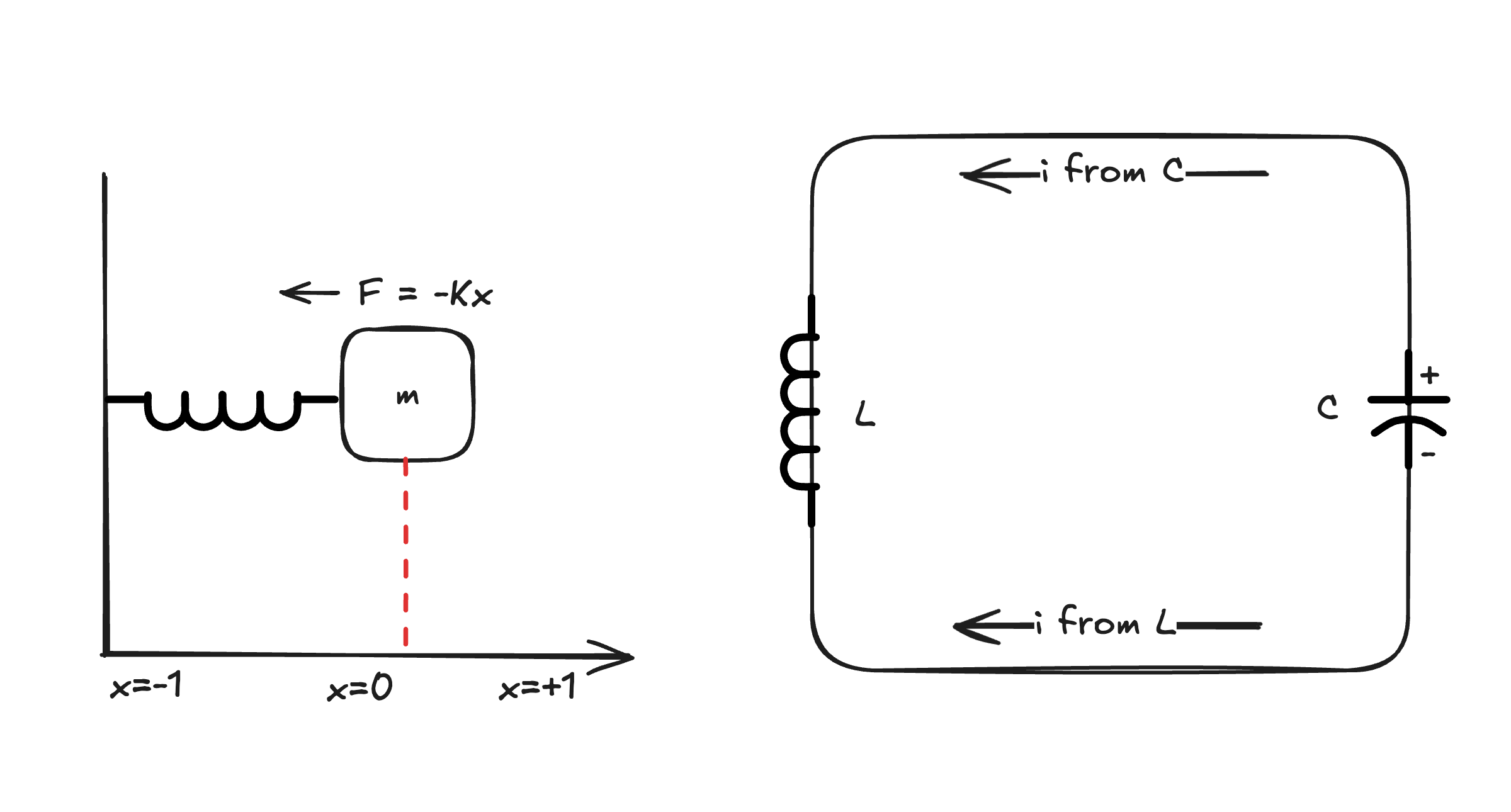
A weight on a spring has a mathematical similarity with an electrical circuit consisting of a capacitor and inductor (LC circuit). They are both examples of harmonic oscillators which exhibit a sinusoidal behavior through time.

Lagrange & Hamiltonian Review

Briefly, the Lagrangian is the difference of kinetic and potential energy ($T$ and $V$ respectively):

\[\mathcal L = T - V\]

More accurately, the Lagrangian is any function that accurately describes a physical law when inputting it into the Euler Lagrange equations:

\[\frac{\partial \mathcal L}{\partial x} - \frac{d}{dt} \frac{\partial \mathcal L}{\partial (\frac{dx}{dt})} = 0\]

The Hamiltonian is the total energy in a system:

\[H = T + V\]

And is a reformulation of Lagrangian Mechanics describing the same physical phenomena. If $\frac{dH}{dt} = 0$, then energy is conserved. Hamilton’s equations are the analog of Euler Lagrange equations.

I have written about Lagrangians & Hamiltonians in previous posts (Lagrangians, Hamiltonians, Lagrangians & physics fields), refer to these for more details.

Mechanical Harmonic Oscillator

Given a spring applying a force $F = -Kx$ to a mass $m$¹, we can write the Hamiltonian and Lagrangian as:

\[\begin{align*} H = T + V = \frac{1}{2}m(\frac{dx}{dt})^2 + \frac{1}{2}Kx^2 \\ \mathcal L = T - V = \frac{1}{2}m(\frac{dx}{dt})^2 - \frac{1}{2}Kx^2 \end{align*}\]

Which gives the following Euler Lagrange Equation:

\[\begin{align} \frac{\partial \mathcal L}{\partial x} - \frac{d}{dt} \frac{\partial \mathcal L}{\partial (\frac{dx}{dt})} = -Kx - m \frac{d^2x}{dt^2} = 0 \label{eqn:mechanical_lagrange} \end{align}\]

And can be rewritten into Newton’s second law:

\[-Kx = m \frac{d^2x}{dt^2} \implies \boxed{F = ma}\]

If we were to solve this second order linear differential equation $\eqref{eqn:mechanical_lagrange}$, we would get a wave:

\[\begin{align*} x(t) = A \sin{(\omega t + \phi)} \\ \omega = \sqrt{\frac{K}{m}} \end{align*}\]

Finally, we have energy conservation by showing $\frac{dH}{dt} = 0$:

\[\begin{align*} \frac{dH}{dt} &= \frac{\partial H}{\partial t} + \frac{\partial H}{\partial x}\frac{\partial x}{\partial t} + \frac{\partial H}{\partial (\frac{dx}{dt})} \frac{d^2 x}{dt^2} \\ \frac{dH}{dt} &= 0 + Kx \frac{dx}{dt} + m \frac{dx}{dt} \frac{d^2 x}{dt^2} \\ \frac{dH}{dt} &= \frac{dx}{dt}(Kx + m \frac{d^2 x}{dt^2}) = 0 \end{align*}\]

Where the last equality comes directly from the Euler Lagrange Equation (or Newton’s second law).

Electrical Harmonic Oscillator (LC Circuit)

The LC circuit (or “tank” circuit) will consist of the following elements²

• Capacitor $C$
  • $Q = Cv_C$
  • $\frac{dQ}{dt} = i = C \frac{dv_C}{dt}$
  • $E_C = \frac{1}{2}Cv_C^2$ (Energy of capacitor)
• Inductor $L$
  • $v_L = L \frac{di}{dt}$
  • $E_L =\frac{1}{2}Li^2$ (Energy of inductor)

More on $i$

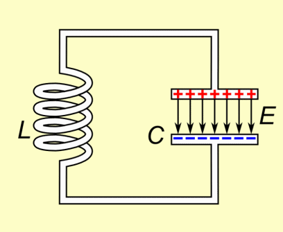
From Lenz’s law we know that the current induced in a circuit due to a change in a magnetic field is directed to oppose the change in flux and to exert a mechanical force which opposes the motion.

Since the capacitor will be sending current through the inductor which creates a magnetic field, the inductor will then have an electromotive force (emf) which affects the capacitor. The following animation from wikipedia visualizes this:

You can read more about this progression here.

For an LC circuit, these components will have the following Hamiltonian:

\[H = \frac{1}{2}Cv_C^2 + \frac{1}{2}Li^2\]

And Lagrangian,

\[\mathcal L = \frac{1}{2}Cv_C^2 - \frac{1}{2}Li^2\]

Unlike in the mechanical example where we had the coordinate system $x$, our energy expressions involve different time-dependent quantities, $v$ and $i$. We can unify the “state” of the system to be the charge $Q$ at time $t$, $Q(t)$.

\[\begin{align*} \mathcal L &= \frac{1}{2}Cv^2 - \frac{1}{2}Li^2 \\ &= \frac{1}{2}C \frac{Q^2}{C^2} - \frac{1}{2}L (\frac{dQ}{dt})^2 \\ &= \frac{1}{2C} Q^2 - \frac{1}{2}L (\frac{dQ}{dt})^2 \end{align*}\]

Now we can apply Euler Lagrange like before to work out the equations of motion:

\[\begin{align} \frac{\partial \mathcal L}{\partial Q} - \frac{d}{dt} \frac{\partial \mathcal L}{\partial (\frac{dQ}{dt})} = \frac{Q}{C} - \frac{d}{dt} (-L\frac{dQ}{dt}) = \frac{Q}{C} + L\frac{d^2Q}{dt^2} = 0 \label{eqn:electric_lagrange} \end{align}\]

Now we will apply the definitions of capacitance and inductance from above:

\[\frac{Q}{C} + L\frac{d^2Q}{dt^2} = \frac{Q}{C} + L\frac{di}{dt} = v_C + v_L = 0\]

Which is Kirchhoff’s voltage law:

\[v_C + v_L = 0 \implies \boxed{\sum_{i=1}^{n}v_i = 0}\]

As before, we can show that the energy of the system is conserved:

\[\begin{align*} H &= \frac{1}{2C} Q^2 + \frac{1}{2}L (\frac{dQ}{dt})^2 \\ \frac{dH}{dt} &= \frac{\partial H}{\partial t} + \frac{\partial H}{\partial Q}\frac{\partial Q}{\partial t} + \frac{\partial H}{\partial (\frac{dQ}{dt})} \frac{d^2 Q}{dt^2} \\ &= \frac{Q}{C}i + L i \frac{d^2 Q}{dt^2} \\ &= i(\frac{Q}{C} + L \frac{d^2 Q}{dt^2}) \\ &= 0 \end{align*}\]

Where the last equality came from the equations of motion.

Relating Electrical and Mechanical Harmonic Oscillators

There is a high degree of similarity between the mechanical and electrical harmonic oscillators,

	Mechanical Oscillator	Electrical Oscillator
Hamiltonian	$\frac{1}{2}m(\frac{dx}{dt})^2 + \frac{1}{2}Kx^2$	$\frac{1}{2}L (\frac{dQ}{dt})^2 + \frac{1}{2} \frac{1}{C} Q^2$
Eqn of Motion	$\frac{d^2}{dt^2}x + \frac{K}{m}x = 0$	$\frac{d^2}{dt^2}q + \frac{1}{LC}q = 0$

With the following substitutions we see they are the same second order differential equation:

• $x \rightarrow Q$
• $m \rightarrow L$
• $K \rightarrow \frac{1}{C}$

As a result, the solution of the LC circuit’s equation of motion must also be a wave:

\[\begin{align*} Q(t) &= A \sin{(\omega t + \phi)} \\ \end{align*}\]

Where $\omega = \sqrt{\frac{1}{LC}}$ is the electrical analog for angular frequency. We can derive the rest of the time dependent quantities:

\[\begin{align*} i(t) &= \frac{dQ(t)}{dt} = \omega A \cos{(\omega t + \phi)} \\ v_L(t) &= L\frac{di}{dt} = -\omega^2 L A \sin{(\omega t + \phi)} \\ v_C(t) &= \frac{Q}{C} = \frac{A}{C} \sin{(\omega t + \phi)} \end{align*}\]

Here is a visualization:

Code Snippet

Beyond LC Circuits

The LC circuit is idealized without any resistance ($R$). In practice, circuits do have resistance and will not conserve energy (losing some energy to heat). We can add $R$ back in to form an RLC circuit which has different expressions for Lagrangian and Hamiltonian. We can further add an A/C voltage source which acts like a driven harmonic oscillator and is used in a variety of frequency filters. You can see how $R$ would affect the LC circuit in this great simulator by Paul Falstad.

References

1. https://eng.libretexts.org/Bookshelves/Electrical_Engineering/Electro-Optics/Direct_Energy_(Mitofsky)/11%3A_Calculus_of_Variations/11.04%3A_Mass_Spring_Example ↩︎

2. https://eng.libretexts.org/Bookshelves/Electrical_Engineering/Electro-Optics/Direct_Energy_(Mitofsky)/11%3A_Calculus_of_Variations/11.05%3A_Capacitor_Inductor_Example ↩︎