Hamiltonian Mechanics

In this post, I discuss the physics behind Hamiltonian Monte Carlo (HMC), Hamiltonian Mechanics.

Hamiltonian Monte Carlo (HMC)

There are several great references for learning about HMC. My favorite is by Radford Neal, here. A concise overview is given by the stan reference manual. I’ll start by quoting their summary:

“The Hamiltonian Monte Carlo algorithm starts at a specified initial set of parameters $\theta$; in Stan, this value is either user-specified or generated randomly. Then, for a given number of iterations, a new momentum vector is sampled and the current value of the parameter $\theta$ is updated using the leapfrog integrator with discretization time $\epsilon$ and number of steps $L$ according to the Hamiltonian dynamics. Then a Metropolis acceptance step is applied, and a decision is made whether to update to the new state $(\theta^∗,\rho^∗)$ or keep the existing state.”

- Stan Manual

Followed by their mathematical description:

\[\begin{gather*} p(\rho, \theta) = p(\rho | \theta)p(\theta) \\ \rho \sim \mathcal N(0, M) \\ \end{gather*}\]

Which forms the Hamiltonian,

\[\begin{flalign*} H(\rho, \theta) &= -\log{p(\rho, \theta)} \\ &= -\log{p(\rho | \theta)} - \log{p(\theta)} \\ &= T(\rho | \theta) + V(\theta) \end{flalign*}\]

That has dynamics described by:

\[\begin{gather*} \frac{d\theta}{dt} = +\frac{\partial H}{\partial \rho} = +\frac{\partial T}{\partial \rho} \\ \frac{d\rho}{dt} = -\frac{\partial H}{\partial \theta} = -\frac{\partial V}{\partial \theta} \end{gather*}\]

There are some practical considerations like using the leapfrog integrator and correcting error with a Metropolis accept step, but at a high level, running these dynamics over time magically yields samples of $\theta$.

And if you don’t believe me, then check out this hw assignment that I completed as part of Stanford’s Stats 271 course. HMC gives similar estimates as MCMC, but with a much higher effective sample size (ESS):

HMC Posterior Trace	HMC Posterior Histogram

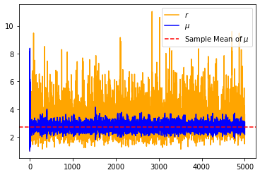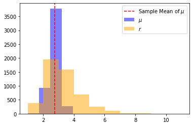Hamiltonian Mechanics

While taking Stats 271, I didn’t have time to look too deeply into the physics formulation. But, building off my recent post about Lagrangian Mechanics, I now have the proper groundwork to understand Hamiltonian Mechanics.

Least Action to Hamiltonian

We start from Least Action and the functional we were seeking to make stationary, the Lagrangian:

\[L(q(t), \dot q(t), t)\]

Where we are back to using $q$ as generalized coordinates (cartesian, polar, etc.) and $\dot q$ is the time derivative, $\frac{dq}{dt}$. Consider the total derivative of this function through time, that is, all the rates of change from having a dependency on time:

\[\begin{flalign*} \frac{dL}{dt} &= \sum_i \frac{\partial L}{\partial q_i} \frac{\partial q_i}{\partial t} + \frac{\partial L}{\partial \dot q_i} \frac{\partial \dot q_i}{\partial t} + \frac{\partial L}{\partial t} \\ &= \sum_i \dot p_i \dot q_i + p_i \ddot q_i + \frac{\partial L}{\partial t} \\ &= \frac{\partial L}{\partial t} + \frac{d}{dt}\sum_i (p_i \dot q_i) \end{flalign*}\]

Where we used the generalized momentum, $p_i = \frac{\partial L}{\partial \dot q_i}$ along with our Euler-Lagrange equation:

\[\frac{\partial L}{\partial q} = \frac{\partial}{\partial t} \frac{\partial L}{\partial \dot q} = \frac{\partial}{\partial t} p_i = \dot p_i\]

in the second line and the product rule of calculus in the third line. Now, let’s define a new quantity and give it a name (more on this later). If,

\[H = \sum_i (p_i \dot q_i) - L\]

Then we would have,

\[\begin{flalign*} \frac{dH}{dt} &= \frac{d}{dt}\sum_i (p_i \dot q_i) - \frac{dL}{dt} \\ &= \frac{d}{dt}\sum_i (p_i \dot q_i) - \frac{\partial L}{\partial t} - \frac{d}{dt}\sum_i (p_i \dot q_i) \\ &= - \frac{\partial L}{\partial t} \\ \end{flalign*}\] \[\begin{equation} \therefore \frac{dH}{dt} = - \frac{\partial L}{\partial t} \label{eqn:hamilton} \end{equation}\]

Which says that the rate of change in $L$, disregarding the contributions from $q$ and $\dot q$, is equal to the opposite of the time derivative of this new quantity $H$. And unlike $L$ which dealt in terms of $q$ and $\dot q$; $H$ deals in terms of $p$ and $q$.

That doesn’t match the HMC dynamics above…

Okay, fair point, but we are close. Now, using our definition of $H$:

\[\begin{gather*} H = \sum_i (p_i \dot q_i) - L(q, \dot q, t) \\ \implies L(q, \dot q, t) + H = \sum_i (p_i \dot q_i) \end{gather*}\]

We can derive the dynamics directly (paying special attention to terms not involving the partial derivatives):

\[\begin{flalign*} \frac{\partial H}{\partial q_i} &= - \frac{\partial L}{\partial q_i} \\ &= - \frac{d}{dt} \frac{\partial L}{\partial \dot q_i} \\ &= -\dot p_i \end{flalign*}\]

Where I again used Euler-Lagrange equations. And very simply,

\[\begin{flalign*} \frac{\partial H}{\partial p_i} &= \dot q_i \end{flalign*}\]

Which gives us the equations:

\[\begin{flalign*} \dot q_i &= \frac{\partial H}{\partial p_i} \\ \dot p_i &= -\frac{\partial H}{\partial q_i} \end{flalign*}\]

Which are the same used by HMC. Speaking of which, why go through all the trouble to apply Hamiltonian Mechanics to MCMC, why not just use Euler Lagrange? What does changing from a system described by $(q, \dot q)$ to $(p, q)$ actually get us? Well instead of solving the $n$-dimensional second order differential equation:

\[\begin{equation*} \frac{\partial L}{\partial q} - \frac{\partial}{\partial t} \frac{\partial L}{\partial \dot q} = 0 \end{equation*}\]

We can solve two $n$-dimensional (coupled) first-order partial differential equations (for a total of $2n$ dimensions).

High School Physics Detour

But what does $H$ physically represent? Let’s go back to our example of $L$ from high school physics:

\[\begin{gather*} L = \frac{m}{2}\dot x^2 - V(x) \\ p = m \dot x \end{gather*}\]

And see what $H$ would be equal to in this case:

\[\begin{flalign*} H &= \sum_i (p_i \dot q_i) - L \\ &= m \dot x \cdot \dot x - \frac{m}{2}\dot x^2 + V(x) \\ &= \frac{m}{2} \dot x^2 + V(x) \\ &= T + V(x) \\ &= E \end{flalign*}\]

$H$ turns out to be the energy of this system. Further:

\[\begin{gather*} \dot p = -\frac{\partial H}{\partial x} = -\frac{\partial V}{\partial x} = F \\ \end{gather*}\] \[\therefore F = m \ddot x\]

Which is Newton’s Second law. So not only does $H$ encode the total energy of our system, but can also tell us the equations of motion.

Legendre Transformation Detour

This transformation from $(q, \dot q)$ space to $(p, q)$ space actually has a name, the Legendre Transformation. Given some conjugate pair $p = \frac{df}{dx}$, the transformation re-expresses:

\[df = \frac{df}{dx}dx = p dx\]

First we define the quantity $f^* = xp - f$ and its derivative:

\[\begin{flalign*} df^* &= d(xp - f) \\ &= d(xp) - df \\ &= pdx + xdp - pdx \\ &= xdp \end{flalign*}\]

This seems uneventful until we apply this transformation to the Lagrangian. We take a conjugate pair with $\dot q$ to transform this variable:

\[\begin{flalign*} f &= L(q, \dot q) \\ x &= q \\ y &= \dot q \\ p &= \frac{\partial f}{\partial y} = \frac{\partial L}{\partial \dot q} \end{flalign*}\]

Then we can directly read off the transformed system,

\[\begin{flalign*} f^* &= y \frac{df}{dy} - f \\ &= p \dot q - L \\ &= H \\ &\implies L + H = p \dot q \end{flalign*}\]

Which is the starting point for when we derived Hamilton’s Equations above. Unsurprsingly, we can derive Hamilton’s equations from $f^*$ and $f$:

$f^*$-

\[\begin{flalign*} \frac{\partial f^*}{\partial p} &= x \\ \implies \frac{\partial H}{\partial p} &= q \end{flalign*}\]

$f$-

\[\begin{flalign*} \frac{\partial f}{\partial x} &= p \\ \implies \frac{\partial L}{\partial q} &= p \\ \implies \frac{\partial (p\dot q - H)}{\partial q} &= p \\ \implies -\frac{\partial H}{\partial q} &= p \end{flalign*}\]

Hamiltonian Properties

The Hamiltonian has a number of properties (matching the presentation of section 2.2) that make it useful:

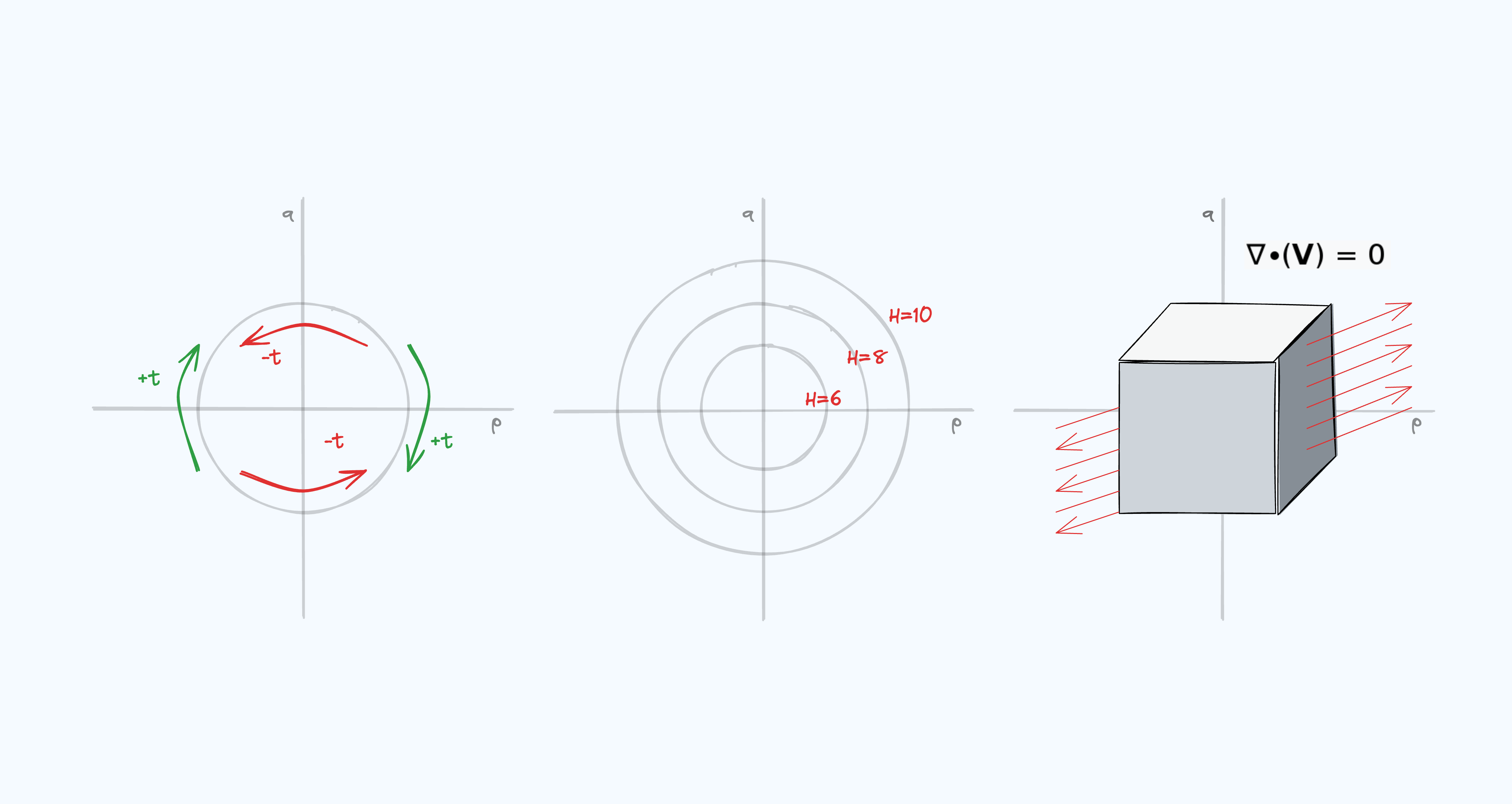
• Reversibility Notice in our high school example that $T$ is a quadratic function of $p$. This is also true in the HMC formulation. From what I can tell, its true in most naturally occurring Hamiltonians (I do not have a citation for this, would be interested to see counter examples). What sort of symmetry does this give us? Consider setting $p \rightarrow -p$:

\[\begin{gather*} -\dot p = -\frac{\partial H}{\partial q} \\ \dot q = \frac{\partial H}{\partial (-p)} = -\frac{\partial H}{\partial p} \end{gather*}\]

Rearranging negative signs further (i.e. $-\dot q = -\frac{\partial q}{\partial t} = \frac{\partial q}{- \partial t}$) would then give us:

\[\begin{gather*} \frac{\partial p}{\partial (-t)} = -\frac{\partial H}{\partial q} \\ -\frac{\partial q}{\partial t} = \frac{\partial q}{\partial (-t)} = -(-\frac{\partial H}{\partial p}) = \frac{\partial H}{\partial p} \end{gather*}\]

Which are the same as the original Hamiltonian equations but with $t \rightarrow -t$. So when we go backwards in the $p$ direction in $(p, q)$ phase space, we follow the exact same equations of motion with $-t$.

• Conservation Consider the case when $L$ is not a function of $t$, i.e. $L(q, \dot q)$ (in one dimension). According to \eqref{eqn:hamilton}, this means that $\frac{\partial L}{\partial t} = 0 \implies \frac{dH}{dt} = 0$. Since $H$ represents the energy of the system, $\frac{dH}{dt} = 0$ means that the energy is conserved. Thus, anytime $L(q, \dot q)$ does not depend on $t$, we know from inspection that the total energy will be conserved. For example, $t$ is not present in $L = \frac{m}{2}\dot x^2 - V(x)$, and thus energy is conserved. This matches what we were taught in high school that potential energy equals kinetic energy when only conservative forces affect the system. Note that this is also the case in our Hamiltonian from HMC.
• Volume Preserving (Liouville’s theorem) If we were to treat the $(q_i, p_i)$ space as a fluid, we would see that it is incompressible. No matter how we squish and reshape the blob, the volume would remain the same. This is shown mathematically with the divergence of a vector $\vec v = [\dot q_1, …, \dot q_n, \dot p_1, …, \dot p_n]$ representing the dynamics of phase space:

\[\begin{flalign*} \nabla \cdot \vec v &= \sum_i (\frac{\partial v_{q_i}}{\partial q_i} + \frac{\partial v_{p_i}}{\partial p_i}) \\ &= \sum_i (\frac{\partial \dot q_i}{\partial q_i} + \frac{\partial \dot p_i}{\partial p_i}) \\ &= \sum_i (\frac{\partial}{\partial q_i} \frac{\partial H}{\partial p_i} - \frac{\partial}{\partial p_i} \frac{\partial H}{\partial q_i}) \\ &= \sum_i (\frac{\partial^2 H}{\partial q_i \partial p_i} - \frac{\partial^2 H}{\partial p_i \partial q_i}) \\ &= 0 \end{flalign*}\]

HMC Revisited

Now we can go back to the HMC example from my Stats271 class, and try to visualize some of these properties. For these plots, I ran HMC for 100 iterations, doing 100 leapfrog steps per iteration.

Conservation

For conservation, we can view the value of the Hamiltonian after each iteration’s leapfrog step:

Phase Space

To visualize the $(p, q)$ phase space, we need two separate plots since the entire vector in this example is $[q_1, q_2, p_1, p_2]$. Normally, in a HMC trace plot, you only show the last $(p, q)$ state after the leapfrog integrator and acceptance step have been taken. Instead, I logged the trace of each iteration’s leapfrog steps, to show the dynamics of each individual iteration. The height of each sample is equal to $\exp{-H(p, q)}$ which converts the energy function to a probability. I also show the (scaled) kde of the frequency of $(p, q)$, to help see the marginal density of this stepping process.

$(p_1, q_1)$

$(p_2, q_2)$

Plot Summary

We see that the leapfrog estimator (roughly) keeps the value of the Hamiltonian constant within an iteration. Between iterations, $p$ is resampled moving the trace to a different “level” of the log density surface. These are the discrete “steps” inside the $H$ vs. iteration plot on the top, and the mini circles in each of the $(p, q)$ phase space plots on the bottom. Other things I noticed were:

• The first position coordinate (the first posterior) seems to be more stable than the second.
• Each of leapfrog steps seem to fluctuate slightly in their value of $H(p, q)$, in the shape of a saddle.

Code for the plots

If you want to see an entire HMC code example, including the interactive plots, please see hw_3 of the blog_post branch in my Stats271 repo here.