Diffusion MNIST with Flux ML (Julia)
Model Info
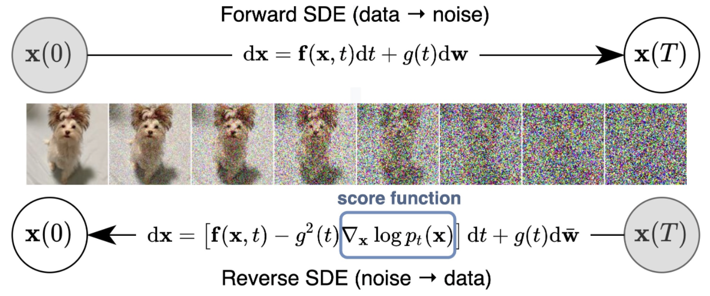
Score-Based Generative Modeling is a framework to learn stochastic dynamics that transitions one distribution to another. In our case, we will be modeling the transition from the MNIST image distribution into random noise. The general idea is to learn the forward dynamics (score function or gradients) of the image’s distribution being slowly evolved into random gaussian noise through a diffusion process. This is shown in the image above with the Forward Stochastic Differential Equation (SDE). With estimates of how the forward dynamics works, we can then reverse the process allowing us to create realistic looking images from pure noise! This is shown with the Reverse SDE in the graphic above.
In contrast to likelihood based models, Score-Based Generative Modeling depends only on the score function, $\nabla_x \log{p(x)}$ which is minimized through score matching. Concretely, this tutorial will be using a UNet architecture and score matching loss function to learn this score function. After this gradient is estimated, we can then draw samples from the MNIST dataset using Langevin Dynamics of the reverse SDE.
More Model Info
A much more in-depth walkthrough of the theory is available here from the original author, Yang Song. I highly recommend this blog to become more familiar with the concepts before diving into the code!
Pytorch Equivalent Code
For those coming from Python, here is the equivalent Pytorch code that was used to create this Julia tutorial.
Training
1
2
cd vision/diffusion_mnist
julia --project diffusion_mnist.jl
Visualization
1
2
cd vision/diffusion_mnist
julia --project diffusion_plot.jl
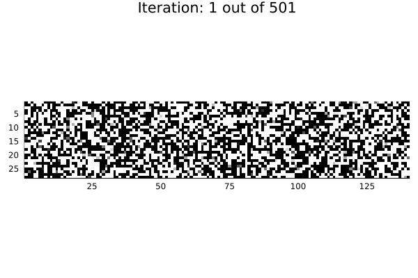
Visualizations are sampled with either the equations used in the original PyTorch tutorial or with the help of DifferentialEquations.jl.
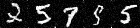
| Sampled Noise | Euler-Maruyama (EM) Sampler | Predictor Corrector Sampler |
|---|---|---|
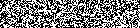 | 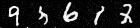 |  |
Euler-Maruyama (DifferentialEquations.jl) | Probability Flow ODE (DifferentialEquations.jl) |
|---|---|
 |  |
And since the DifferentialEquations.jl’s solve() returns the entire sample path, it is easy to visualize the reverse-time SDE sampling process as an animation:
| Euler-Maruyama | Probability Flow ODE |
|---|---|
 |  |
And finally, we can visualize the components of the image, 𝙭, as a function of t ∈ [1, ϵ]. As noted by the authors, the Probability Flow ODE captures the same marginal probability density 𝒫ₜ(𝙭) as it’s stochastic counterpart.
 | 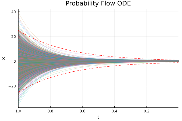 |
The lines, x(t) = ± σᵗ, are shown for reference.