Bayesian Optimization in BoTorch

BoTorch is the python library behind the Ax engine I was using in my previous blog. I enjoyed making that post so much that I decided to take a deep dive into making custom models with the Model and Posterior API. Enjoy!

Custom Models in BoTorch

In this tutorial, we illustrate how to create a custom surrogate model using the Model and Posterior interface. We will cover creating surrogate models from:

• PyTorch distributions
• Posterior samples (using Pyro)
• Ensemble of ML predictions

This tutorial differs from the Using a custom BoTorch model with Ax tutorial by focusing more on authoring a new model that is compatible with the BoTorch and less on integrating a custom model with Ax’s botorch_modular API.

import torch

# Set the seed for reproducibility
torch.manual_seed(1)
# Double precision is highly recommended for BoTorch.
# See https://github.com/pytorch/botorch/discussions/1444
torch.set_default_dtype(torch.float64)

train_X = torch.rand(20, 2) * 2
Y = 1 - (train_X - 0.5).norm(dim=-1, keepdim=True)
Y += 0.1 * torch.rand_like(Y)
bounds = torch.stack([torch.zeros(2), 2 * torch.ones(2)])

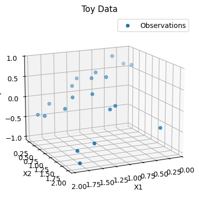
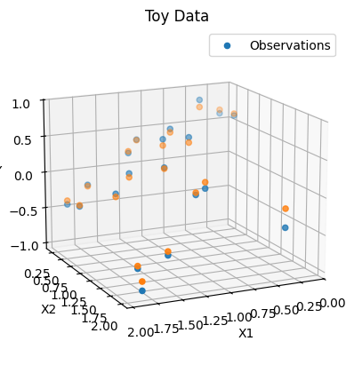
Code to plot our training data.

from matplotlib import pyplot as plt
from matplotlib.axes import Axes
from torch import Tensor
from mpl_toolkits.mplot3d import Axes3D

# Needed for older versions of matplotlib.
assert Axes3D


def plot_toy_data(x: Tensor, y: Tensor) -> Axes:
    ax = plt.figure().add_subplot(projection="3d")
    ax.scatter(
        x[:, 0].detach().numpy().squeeze(),
        x[:, 1].detach().numpy().squeeze(),
        zs=y.detach().numpy().squeeze(),
        label="Observations",
    )
    ax.set_xlabel("X1")
    ax.set_ylabel("X2")
    ax.set_zlabel("Y")
    ax.set_title("Toy Data")
    ax.view_init(elev=15.0, azim=65)
    ax.legend()
    return ax


plot_toy_data(x=train_X, y=Y)
plt.show()

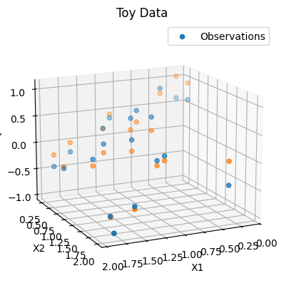
Probabilistic Linear Regression (w/ Torch Distributions)

BoTorch’s Model class only requires you to define a posterior() method that returns a Posterior object, the only requirement of which is to implement an rsample() function for drawing posterior samples. Specifically, we can utilize the subclass TorchPosterior that directly wraps a torch distribution.

from typing import Optional, Union
from torch import Tensor, distributions, nn
from botorch.acquisition.objective import PosteriorTransform
from botorch.models.model import Model
from botorch.posteriors.posterior import Posterior
from botorch.posteriors.torch import TorchPosterior


class ProbabilisticRegressionModel(Model):
    _num_outputs: int

    def __init__(self, train_X: Tensor, train_Y: Tensor):
        super(ProbabilisticRegressionModel, self).__init__()
        self._num_outputs = train_Y.shape[-1]
        # Linear layer that will compute the regression output.
        self.linear = nn.Linear(train_X.shape[-1], self.num_outputs)

    @property
    def num_outputs(self) -> int:
        return self._num_outputs

    def forward(self, x: Tensor) -> distributions.Distribution:
        n, p = x.squeeze().shape
        # For now, let's suppose we have known variance 1.
        return distributions.StudentT(df=n - p, loc=self.linear(x), scale=1)

    def posterior(
        self,
        X: Tensor,
        output_indices: Optional[list[int]] = None,
        observation_noise: Union[bool, Tensor] = False,
        posterior_transform: Optional[PosteriorTransform] = None,
    ) -> Posterior:
        if output_indices:
            X = X[..., output_indices]
        # TorchPosterior directly wraps our torch.distributions.Distribution output.
        posterior = TorchPosterior(distribution=self(X))
        if posterior_transform is not None:
            posterior = posterior_transform(posterior)
        return posterior

[KeOps] Warning : omp.h header is not in the path, disabling OpenMP. To fix this, you can set the environment
                  variable OMP_PATH to the location of the header before importing keopscore or pykeops,
                  e.g. using os.environ: import os; os.environ['OMP_PATH'] = '/path/to/omp/header'
[KeOps] Warning : Cuda libraries were not detected on the system or could not be loaded ; using cpu only mode

def fit_prob_reg(
    epochs: int,
    model: ProbabilisticRegressionModel,
    optimizer: torch.optim.Optimizer,
    train_X: Tensor,
    train_Y: Tensor,
) -> None:
    """Optimization loop for linear regression."""
    train_X = train_X.requires_grad_()
    for epoch in range(epochs):
        optimizer.zero_grad()
        outputs = model(train_X)
        loss = -outputs.log_prob(train_Y).mean()
        loss.backward()
        optimizer.step()
        if epoch % 10 == 0:
            print("epoch {}, loss {}".format(epoch, loss.item()))

prob_regression_model = ProbabilisticRegressionModel(train_X, Y)
optimizer = torch.optim.Adam(prob_regression_model.parameters(), lr=0.1)
fit_prob_reg(50, prob_regression_model, optimizer, train_X, Y)

epoch 0, loss 1.3283335654335957
epoch 10, loss 1.0691577720241896
epoch 20, loss 0.9760611872620313
epoch 30, loss 0.9548081485136333
epoch 40, loss 0.9551388835842956

ax = plot_toy_data(x=train_X, y=Y)
ax.scatter(
    train_X[:, 0].detach().numpy().squeeze(),
    train_X[:, 1].detach().numpy().squeeze(),
    zs=prob_regression_model(train_X).mean.detach().squeeze().numpy(),
)
plt.show()

Finally, since our custom model is based off Model and Posterior, we can use both analytic and MC based acquisition functions for optimization.

from botorch.acquisition.analytic import LogExpectedImprovement
from botorch.optim.optimize import optimize_acqf

candidate, acq_val = optimize_acqf(
    LogExpectedImprovement(model=prob_regression_model, best_f=Y.max()),
    bounds=bounds,
    q=1,
    num_restarts=5,
    raw_samples=10,
)
candidate, acq_val

(tensor([[0., 0.]]), tensor(-0.1007))

Before using qLogExpectedImprovement we need to register an appropriate sampler for the TorchPosterior. We can use the following code to create a MCSampler for that is specific to torch.distributions.StudentT.

from botorch.sampling.base import MCSampler
from botorch.sampling.get_sampler import GetSampler
from botorch.sampling.stochastic_samplers import ForkedRNGSampler


@GetSampler.register(distributions.StudentT)
def _get_sampler_torch(
    posterior: TorchPosterior,
    sample_shape: torch.Size,
    *,
    seed: Optional[int] = None,
) -> MCSampler:
    # Use `ForkedRNGSampler` to ensure determinism in acquisition function evaluations.
    return ForkedRNGSampler(sample_shape=sample_shape, seed=seed)

from botorch.acquisition.logei import qLogExpectedImprovement

optimize_acqf(
    qLogExpectedImprovement(model=prob_regression_model, best_f=Y.max()),
    bounds=bounds,
    q=1,
    num_restarts=5,
    raw_samples=10,
)

(tensor([[0., 0.]]), tensor(-0.1105))

Supported PyTorch Distributions

Although we chose the StudentT distribution in the above example, any distribution supporting the rsample method will work with BoTorch’s automatic differentiation. We can use the has_rsample attribute to see a complete listing of compatible distributions.

print(
    [
        j.__name__
        for j in [getattr(distributions, i) for i in distributions.__all__]
        if hasattr(j, "has_rsample") and j.has_rsample
    ]
)

['Beta', 'Cauchy', 'Chi2', 'ContinuousBernoulli', 'Dirichlet', 'Exponential', 'FisherSnedecor', 'Gamma', 'Gumbel', 'HalfCauchy', 'HalfNormal', 'Independent', 'InverseGamma', 'Kumaraswamy', 'Laplace', 'LogNormal', 'LogisticNormal', 'LowRankMultivariateNormal', 'MultivariateNormal', 'Normal', 'OneHotCategoricalStraightThrough', 'Pareto', 'RelaxedBernoulli', 'RelaxedOneHotCategorical', 'StudentT', 'Uniform', 'Weibull', 'Wishart', 'TransformedDistribution']

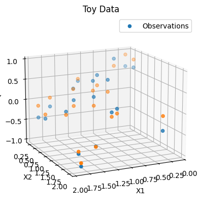
Bayesian Linear Regression

In the previous section, we directly parameterized a “posterior” with a linear layer. In this section, we will follow Chapter 14.2 of Bayesian Data Analysis to implement a proper posterior analytically. This implementation also uses TorchPosterior and the StudentT distribution like before.

from typing import Optional, Union
from torch import Tensor, distributions, nn
from botorch.acquisition.objective import PosteriorTransform
from botorch.models.model import Model
from botorch.posteriors.posterior import Posterior
from botorch.posteriors.torch import TorchPosterior


def add_intercept(x: Tensor) -> Tensor:
    """Adds an intercept column to the design matrix (i.e. tensor)."""
    return torch.concat([torch.ones_like(x)[..., 0:1], x], dim=-1)


class BayesianRegressionModel(Model):
    _num_outputs: int
    df: int
    s_squared: Tensor
    beta: Tensor
    L: Tensor
    add_intercept: bool

    def __init__(self, intercept: bool = True) -> None:
        super(BayesianRegressionModel, self).__init__()
        self.add_intercept = intercept

    @property
    def num_outputs(self) -> int:
        return self._num_outputs

    def forward(self, x: Tensor) -> Tensor:
        return x @ self.beta

    def fit(self, x: Tensor, y: Tensor) -> None:
        self._num_outputs = y.shape[-1]
        x = add_intercept(x) if self.add_intercept else x
        n, p = x.shape
        self.df = n - p
        # Rather than V = torch.linalg.inv(x.T @ x) as in BDA
        # instead use L = torch.linalg.cholesky(x.T @ x) for stability.
        # To use L, we can simply replace operations like:
        # x = V @ b
        # with a call to `torch.cholesky_solve`:
        # x = torch.cholesky_solve(b, L)
        self.L = torch.linalg.cholesky(x.T @ x)
        # Least squares estimate
        # self.beta = torch.cholesky_solve(x.T, self.L) @ y
        self.beta = torch.cholesky_solve(x.T, self.L) @ y
        # Model's residuals from the labels.
        r: Tensor = y - self(x)
        # Sample variance
        self.s_squared = (1 / self.df) * r.T @ r

    def posterior(
        self,
        X: Tensor,
        output_indices: Optional[list[int]] = None,
        observation_noise: Union[bool, Tensor] = False,
        posterior_transform: Optional[PosteriorTransform] = None,
    ) -> Posterior:
        # Squeeze out the q dimension if needed.
        n, q, _ = X.shape
        if output_indices:
            X = X[..., output_indices]
        if self.add_intercept:
            X = add_intercept(X)
        loc = self(X)
        # Full covariance matrix of all test points.
        cov = self.s_squared * (
            torch.eye(n, n) + X.squeeze() @ torch.cholesky_solve(X.squeeze().T, self.L)
        )
        # The batch semantics of BoTorch evaluate each data point in their own batch.
        # So, we extract the diagonal representing Var[\tilde y_i | y_i] of each test point.
        scale = torch.diag(cov).reshape(n, q, self.num_outputs)
        # Form the posterior predictive dist according to Sec 14.2, Pg 357 of BDA.
        posterior_predictive_dist = distributions.StudentT(
            df=self.df, loc=loc, scale=scale
        )
        posterior = TorchPosterior(distribution=posterior_predictive_dist)
        if posterior_transform is not None:
            posterior = posterior_transform(posterior)
        return posterior

bayesian_regression_model = BayesianRegressionModel(intercept=True)
bayesian_regression_model.fit(train_X, Y)

ax = plot_toy_data(x=train_X, y=Y)
ax.scatter(
    train_X[:, 0].detach().numpy().squeeze(),
    train_X[:, 1].detach().numpy().squeeze(),
    zs=bayesian_regression_model(add_intercept(train_X)).detach().squeeze().numpy(),
)
plt.show()

optimize_acqf(
    LogExpectedImprovement(model=bayesian_regression_model, best_f=Y.max()),
    bounds=bounds,
    q=1,
    num_restarts=5,
    raw_samples=10,
)

(tensor([[0., 0.]]), tensor(-1.3847))

optimize_acqf(
    qLogExpectedImprovement(model=bayesian_regression_model, best_f=Y.max()),
    bounds=bounds,
    q=1,
    num_restarts=5,
    raw_samples=10,
)

(tensor([[0., 0.]]), tensor(-1.3684))

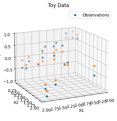
Bayesian Linear Regression w/ EnsemblePosterior

The EnsembleModel class provides a default implementation for posterior(). Then the MC acquisition function will be optimized using samples from the posterior predictive distribution (EnsemblePosterior also implements mean and variance properties, so some other analytic acquisition functions will also work). We follow this Pyro tutorial for a linear regression model fit with Stochastic Variational Inference (SVI).

First, we define a Pyro model capable of sampling from a posterior predictive distribution for new observations at test points. Later, when we perform posterior predictive inference, we will use Pyro’s Predictive class. By default, Predictive ignores inference gradients with:

model = torch.no_grad()(poutine.mask(model, mask=False) if mask else model)

Since we need to retain the autograd graph to optimize the acquisition function, we can use torch.set_grad_enabled(True) in the forward() method to override this behavior.

import pyro
import pyro.distributions as dist
from pyro.infer.autoguide import AutoGuide, AutoDiagonalNormal
from pyro.nn import PyroSample, PyroModule
from pyro.infer import SVI, Trace_ELBO
from pyro.optim import PyroOptim

pyro.set_rng_seed(1)


# Bayesian Regression represented as a single hidden layer.
class BayesianRegression(PyroModule):
    Y: str = "y"

    def __init__(self, in_features: int, out_features: int):
        super().__init__()
        # Linear layer like before, but wrapped with PyroModule.
        self.linear = PyroModule[nn.Linear](in_features, out_features)
        # Add priors to the weights & bias of the linear layer.
        self.linear.weight = PyroSample(
            dist.Normal(0.0, 1.0)
            .expand(torch.Size([out_features, in_features]))
            .to_event(2)
        )
        self.linear.bias = PyroSample(
            dist.Normal(0.0, 10.0).expand(torch.Size([out_features])).to_event(1)
        )

    def forward(self, x: Tensor, y: Optional[Tensor] = None) -> Tensor:
        # NOTE: Enable gradient tracking to override behavior of `Predictive`.
        torch.set_grad_enabled(True)
        # Prior for the noise level.
        sigma = pyro.sample("sigma", dist.Uniform(0.0, 10.0))
        # Linear layer on the inputs.
        mean = self.linear(x).squeeze(-1)
        n, p = x.shape[0], x.shape[-1]
        with pyro.plate("data", x.shape[0]):
            # Observations will be t distributed.
            t_dist = dist.StudentT(df=n - p, loc=mean, scale=sigma)
            _ = pyro.sample(self.Y, t_dist, obs=y)
        return mean

def fit_svi(
    epochs: int,
    model: PyroModule,
    guide: AutoGuide,
    optimizer: PyroOptim,
    train_X: Tensor,
    train_Y: Tensor,
) -> None:
    svi = SVI(
        model,
        guide,
        optimizer,
        loss=Trace_ELBO(),
    )
    pyro.clear_param_store()
    for epoch in range(epochs):
        loss = svi.step(train_X, train_Y.squeeze())
        if epoch % 10 == 0:
            print("epoch {}, loss {}".format(epoch, loss))

Now, we incorporate our Pyro model into the Model and Posterior interface like before. EnsemblePosterior expects a (b) x s x q x m tensor where m is the output size of the model and s is the ensemble size.

from botorch.models.ensemble import EnsembleModel
from pyro.infer import Predictive

class EnsembleBayesianRegressionModel(EnsembleModel):
    model: BayesianRegression
    guide: AutoGuide
    num_samples: int
    _num_outputs: int

    def __init__(self, train_X: Tensor, train_Y: Tensor, num_samples: int = 100):
        super(EnsembleBayesianRegressionModel, self).__init__()
        self._num_outputs = train_Y.shape[-1]
        self.model = BayesianRegression(train_X.shape[-1], self.num_outputs)
        self.guide = AutoDiagonalNormal(self.model)
        self.num_samples = num_samples

    def forward(self, X: Tensor) -> Tensor:
        predictive = Predictive(
            self.model,
            guide=self.guide,
            num_samples=self.num_samples,
            # Only return the posterior predictive distribution for y.
            return_sites=(self.model.Y,),
        )
        # `EnsemblePosterior` expects a `(b) x s x q x m` tensor where `m` is the
        # output size of the model and `s` is the ensemble size.
        samples = (
            # Retrieve posterior samples from the observation random variable.
            # This is also known as a posterior predictive distribution.
            predictive(X.squeeze())[self.model.Y]
            # Move the ensemble dimension to "s" axis.
            .transpose(0, 1)
            # Reshape for `EnsemblePosterior` as mentioned above.
            .reshape(X.shape[0], -1, 1, self.num_outputs)
        )
        return samples

ensemble_bayesian_regression_model = EnsembleBayesianRegressionModel(
    train_X=train_X, train_Y=Y
)
fit_svi(
    100,
    ensemble_bayesian_regression_model.model,
    ensemble_bayesian_regression_model.guide,
    pyro.optim.Adam({"lr": 0.1}),
    train_X,
    Y,
)

epoch 0, loss 57.859971924474735
epoch 10, loss 47.17245571053782
epoch 20, loss 27.547291517941602
epoch 30, loss 34.39363837327427
epoch 40, loss 43.94011251783476
epoch 50, loss 33.11519462561163
epoch 60, loss 28.7194289840763
epoch 70, loss 24.450418378181947
epoch 80, loss 11.057529271793364
epoch 90, loss 13.638860647173294

ax = plot_toy_data(x=train_X, y=Y)
ax.scatter(
    train_X[:, 0].detach().numpy().squeeze(),
    train_X[:, 1].detach().numpy().squeeze(),
    zs=ensemble_bayesian_regression_model(train_X)
    .detach()
    .squeeze()
    .mean(dim=-1)
    .numpy(),
)
plt.show()

optimize_acqf(
    LogExpectedImprovement(model=ensemble_bayesian_regression_model, best_f=Y.max()),
    bounds=bounds,
    q=1,
    num_restarts=5,
    raw_samples=10,
)

(tensor([[0., 0.]]), tensor(-1.0121))

optimize_acqf(
    qLogExpectedImprovement(model=ensemble_bayesian_regression_model, best_f=Y.max()),
    bounds=bounds,
    q=1,
    num_restarts=5,
    raw_samples=10,
)

(tensor([[0., 0.]]), tensor(-0.8815))

Random Forest w/ Ensemble Posterior

Finally, we move away from linear models to any ML technique that ensembles many models. Specifically, we can use the RandomForestRegressor from sklearn which is an ensemble method of individual decision trees. These decision trees can be accessed through the object’s estimators_ attribute.

import numpy as np
from sklearn.ensemble import RandomForestRegressor
from botorch.models.ensemble import EnsembleModel


class EnsembleRandomForestModel(EnsembleModel):
    model: RandomForestRegressor
    num_samples: int
    _num_outputs: int

    def __init__(self, num_samples: int = 100):
        super(EnsembleRandomForestModel, self).__init__()
        self._num_outputs = 1
        self.model = RandomForestRegressor(n_estimators=num_samples)

    def fit(self, X: Tensor, y: Tensor) -> None:
        self.model = self.model.fit(
            X=X.detach().numpy(), y=y.detach().numpy().squeeze()
        )

    def forward(self, X: Tensor) -> Tensor:
        x = X.detach().numpy().squeeze()
        # Create the ensemble from predictions from each decision tree.
        y = torch.from_numpy(np.array([i.predict(x) for i in self.model.estimators_]))
        # `EnsemblePosterior` expects a `(b) x s x q x m` tensor where `m` is the
        # output size of the model and `s` is the ensemble size.
        samples = y.transpose(0, 1).reshape(X.shape[0], -1, 1, self.num_outputs)
        return samples

ensemble_random_forest_model = EnsembleRandomForestModel(num_samples=300)
ensemble_random_forest_model.fit(X=train_X, y=Y)

ax = plot_toy_data(x=train_X, y=Y)
ax.scatter(
    train_X[:, 0].detach().numpy().squeeze(),
    train_X[:, 1].detach().numpy().squeeze(),
    zs=ensemble_random_forest_model(train_X).detach().squeeze().mean(dim=-1).numpy(),
)
plt.show()

In order to use gradient-based optimization of the acquisition function (via the standard optimize_acqf() method) we will need to have the samples drawn from the posterior be differentiable w.r.t. to the input to the posterior() method (this is not the case for Random Forest models). Instead, we will perform the acquisition function optimization with gradient-free methods.

optimize_acqf(
    LogExpectedImprovement(model=ensemble_random_forest_model, best_f=Y.max()),
    bounds=bounds,
    q=1,
    num_restarts=5,
    raw_samples=10,
    options={"with_grad": False},
)

(tensor([[0.3959, 1.3023]]), tensor(-4.3914))

optimize_acqf(
    qLogExpectedImprovement(model=ensemble_random_forest_model, best_f=Y.max()),
    bounds=bounds,
    q=1,
    num_restarts=5,
    raw_samples=10,
    options={"with_grad": False},
)

(tensor([[0.9057, 0.0959]]), tensor(-15.1323))

CMA-ES

We can also move the optimization loop out of BoTorch entirely and follow the CMA-ES tutorial to optimize with an evolution strategy.

import cma
import numpy as np

x0 = np.random.rand(2)

es = cma.CMAEvolutionStrategy(
    x0=x0,
    sigma0=0.2,
    inopts={"bounds": [0, 2], "popsize": 50},
)

log_expected_improvement_ensemble_random_forest_model = LogExpectedImprovement(
    model=ensemble_random_forest_model, best_f=Y.max()
)

with torch.no_grad():
    while not es.stop():
        xs = es.ask()
        y = (
            -log_expected_improvement_ensemble_random_forest_model(
                torch.from_numpy(np.array(xs)).unsqueeze(-2)
            )
            .view(-1)
            .double()
            .numpy()
        )
        es.tell(xs, y)

torch.from_numpy(es.best.x)

(25_w,50)-aCMA-ES (mu_w=14.0,w_1=14%) in dimension 2 (seed=380612, Wed Aug 21 17:25:36 2024)





tensor([0.4497, 0.8411])